Cauchy's Theorem for Rectifiable Jordan Curves

I’d far rather be happy than right any day, Douglas Adams, The Hitchhiker’s Guide to the Galaxy.

Introduction

A complex function $f(z)$ maps $z = x + iy \in \mathbb{C}$ to another complex number. For example: $f(z) = z^2 = (x + iy)^2 = x^2 - y^2 + 2ixy, f(z) = \frac{1}{z}, f(z) = \sqrt{z^2 + 7}$.

A contour is a continuous, piecewise-smooth curve defined parametrically as: $z(t) = x(t) + iy(t), \quad a \leq t \leq b$.

Definition (Smooth Contour Integral). Let ᵞ be a smooth contour (a continuously differentiable path in the complex plane), $\gamma: [a, b] \to \mathbb{C}$. Let $f: \gamma^* \to \mathbb{C}$ be a continuous complex-valued function defined on the trace $\gamma^*$ of the contour (i.e. along the image of $\gamma$). Then, the contour integral of f along $\gamma$ is defined as $\int_{\gamma} f(z)dz := \int_{a}^{b} f(\gamma(t)) \gamma^{'}(t)dt$.

Properties

• Cauchy Integral Formula. If a function f is analytic in a simply connected domain D and γ is a simply closed contour (positive orientated) in D. Then, for any point $z_0$ inside γ we have $f(z_0) = \frac{1}{2\pi i}\cdot \int_{\gamma} \frac{f(z)}{z-z_0}dz$ (Figure D).

• The Residue Theorem states that the integral of a function f(z) around a simple (doesn't cross itself), and positively oriented (counter-clockwise) contour γ is equal to 2πi times the sum of the residues of all singularities inside the contour, $\int_{\gamma} f(z)dz = 2\pi i \sum Res(f, z_k)$ where $z_k$ is a reside inside γ. f must be analytic inside the contour γ, except for a finite number of isolated singularities.

1. For a simple pole at a point $z_k$ (i.e., the denominator has a simple root) is calculated using the formula $Res(f, z_k) = \lim_{z \to z_k}(z-z_k)f(z)$.
2. For a pole of order m, $Res(f, z_k) = \frac{1}{(m-1)!}\lim_{z \to z_k} \frac{d^{m-1}}{dz^{m-1}}[(z-z_k)^mf(z)]$

• Proposition. Linearity of the contour integral, $\int_{\gamma} (af(z) + bg(z))dz = a\int_{\gamma} f(z)dz + b\int_{\gamma} g(z)dz$
• Proposition. Properties of contour integrals under path manipulation. Let γ be a contour, defined by a function $\gamma: [a, b] \to \mathbb{C}$ and let f be a continuous functions $f: \gamma^* \to \mathbb{C}$ defined along the image of ᵞ. Then,

1. Reversal of orientation. $\int_{-\gamma} f(z)dz = -\int_{\gamma} f(z)dz$ where $-\gamma:[a,b] \to \mathbb{C}$ is the reverse of the contour (traversing the same path in the opposite direction) defined by $(- \gamma)(t)=\gamma(a+b-t)$. This property states that reversing the direction of a contour changes or flips the sign of the integral. Intuitively, this is analogous to how reversing the limits of integration in real analysis changes the sign: $\int_a^b f(x)dx = -\int_b^a f(x)dx$. In complex analysis, the orientation of the contour matters because the integral depends on the direction in which we traverse the path.
2. Additivity under subdivision. Suppose a < c < b, let split $\gamma$ into two sub-contours $\gamma_1 = \gamma|_{[a, c]} \text{ and } \gamma_2 = \gamma|_{[c, b]}$, then $\int_{\gamma} f(z)dz = \int_{\gamma_1} f(z)dz + \int_{\gamma_2} f(z)dz$. This property states that integrating over the whole contour is the same as integrating over the pieces successively. This is the complex analogue of the additive property of definite integrals: $\int_a^b f(x)dx = \int_a^c f(x)dx + \int_c^b f(x)dx $ for a < c < b.
3. Invariance of Contour Integrals Under Reparameterization. Let $\tilde{\gamma}$ be a contour, defined by a function $\tilde{\gamma}: [c, d] \to \mathbb{C}$. If $\tilde{\gamma}$ is another parameterization of the same oriented path $\gamma$ meaning there exists a one-to-one, continuously differentiable map $\psi: [c,d]\to[a,b]$ with a positive derivative $\psi'(t)>0$ such that $\tilde{\gamma}(t) = \gamma(\psi(t))$, then $\int_{\gamma} f(z)dz = \int_{\tilde{\gamma}} f(z)dz$

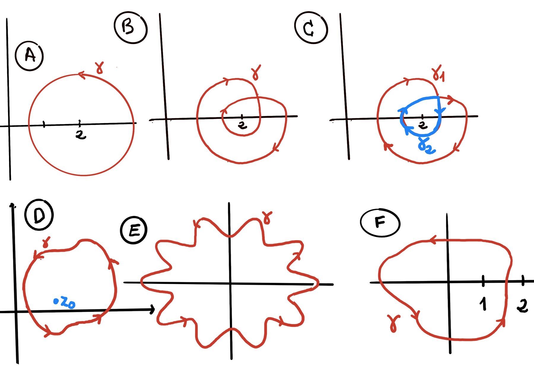
• Deformation of Contours. If two contours $\gamma_1$ and $\gamma_2 $ are homotopic (i.e., one can be continuously deformed into the other without crossing any singularities of f) in a domain where f(z) is analytic, then: $\int_{\gamma_1} f(z)dz = \int_{\gamma_2} f(z)dz.$

• Fundamental Theorem of Calculus for Contours. Suppose $\gamma$ is a contour (piecewise smooth path) from a to b, f is defined on a domain D containing $\gamma^*$ (the image of $\gamma$) and admits a primitive (antiderivative) F on D (i.e., $F'(z) = f(z)$), then $\int_{\gamma} f(z)dz = F(\gamma(b)) - F(\gamma(a))$. In particular, if $\gamma$ is a closed contour (i.e., $\gamma(a)=\gamma(b)$), this integral evaluates to zero, $\int_{\gamma} f(z)dz = 0.$

• Estimation Theorem or the Triangle Inequality for Integrals. The triangle inequality for integrals in complex analysis states thatfor any continuous complex function $f:[a,b] \to \mathbb{C}$ on a closed real interval [a,b] (f(t) = u(t) + iv(t), t a real parameter), the following holds: $∣\int_a^b f(t)dt| \leq \int_a^b |f(t)|dt$.

• Estimation Lemma (ML Inequality) for contour integrals. For any continuous complex function $f:[a,b] \to \mathbb{C}$ on a closed real interval [a,b] (f(z) = u(x, y) + iv(x, y)) with f bounded by some constant M along the entire contour, |f(z)| ≤ M for all $z \in \gamma^*$ (the image/trace of the contour in the complex plane), the following holds: $∣\int_\gamma f(z)dz| \leq M \cdot l(\gamma)$ where l(γ) is the arc length of the contour γ given by $\int_a^b |\gamma^{'}(t)|dt = \int_a^b \sqrt{x'(t)^2 + y'(t)^2} \text{ where } \gamma(t) = x(t) + iy(t)$.

Cauchy’s Theorem in Complex Analysis

• Cauchy’s theorem (Classical “Green’s theorem” version). Let $\Omega \subset \mathbb{C}$ be an open domain. Suppose f = u + iv is analytic in $\Omega$ and its partial derivatives ( $u_x,u_y,v_x,v_y$) are continuous in $\Omega$. If $\gamma$ is a positively oriented, piecewise-smooth $C^1$, simple closed contour with $\gamma^* \cup \operatorname{Int}(\gamma) \subset \Omega$ (its path and interior both lie inside Ω), then $\oint_{\gamma} f(z)dz = 0.$

• Cauchy’s Theorem (Cauchy–Goursat). This is the more powerful version, as it removes the need for continuous partial derivatives. If f is analytic in an open set containing a simple closed contour γ and its interior $\gamma^*\cup\operatorname{Int}(\gamma)$, then $\oint_{\gamma} f(z)dz = 0$.

Rectifiable Jordan curves

Definition. A rectifiable Jordan curve is a curve $\gamma$ in the complex plane satisfying four key properties:

• γ is Simple: The curve does not intersect itself. Formally, if $\gamma: [a, b] \to \mathbb{C}$ is a parameterization, then $\gamma$ is injective on the half-open interval [a, b).
• γ is Closed: The curve returns exactly to its starting point. In other words, it forms a complete loop, starting and ending at the same point. Formally, $\gamma(a)=\gamma(b)$.
• γ is rectifiable if its arc length is finite. This means that, regardless of the curve’s shape (smooth, piecewise smooth, or otherwise “tame”), the process of measuring its length as the “sum” of infinitesimal increments yields a finite value. The arc length of a curve is defined as the supremum of the lengths of all possible inscribed polygonal paths. For any finite ordered partition π, $a = t_0 < t_1 < \cdots < t_n = b$ of [a, b], the polygonal path joining the points $\gamma(t_0), \gamma(t_1), \ldots, \gamma(t_n)$ has length $L_π(\gamma) = \sum_{i=1}^{n} d(\gamma(t_{i-1}), \gamma(t_i)).$ The total arc length of $\gamma$ is defined as the supremum over all such partitions $\Pi$, $L(\gamma) = \sup_{π∈Π} L_\Pi(\gamma) = \sup_{π\in \Pi} \{ \sum_{i = 1}^n d(\gamma(t_{i-1}), \gamma(t_i)) : a=t_0 < t_1 < \cdots < t_n =b \}$ where the supremum runs over all finite partitions of [a, b].

Rectifiability is automatic if γ is piecewise C¹ (each smooth piece has a continuous derivative) or C¹. This means the curve is composed of a finite number of segments, each of which is continuously differentiable -it has a derivative everywhere, and that derivative is continuous. γ′ ∈ L¹ (it is integrable in the Lebesgue sense: the integral of its absolute value is finite). Corners and cups are allowed; wild fractal oscillations and self-intersections are not.

How to check rectifiability quickly. If $\gamma:[a,b] \to \mathbb{C}$ is piecewise $C^1$ and $\int_a^b |\gamma'(t)|dt < \infty$, then $\gamma$ is rectifiable. If $\gamma$ is a simple polygon or a smooth perturbation of a circle, it’s rectifiable.

The Jordan’s curve theorem

A fundamental result in topology is the Jordan’s curve theorem.

Jordan’s curve theorem. Any simple closed curve divides or separates the complex plane into two disjoint connected regions: one interior (bounded) and one exterior (unbounded). In other words, it partitions the plane into exactly three disjoint sets:

1. The Curve itself ($\gamma$) is the boundary of both regions.
2. The Interior (Int($\gamma$)) is the finite area enclosed by the curve (e.g., if you draw a circle on a piece of paper, the interior region would be everything inside the circle). It is a bounded, simply connected region.
3. The Exterior (Ext($\gamma$)) is the infinite area outside the curve (e.g., using the same circle example, the exterior region would include all points on the paper that are not inside the circle). It is an unbounded region.

Examples:

• Polygons. Simple closed shapes with straight sides (triangles, rectangles, pentagons, etc.) Their length is simply the sum of their side lengths, e.g., a unit square with vertices at 0, 1, 1+i, i.
• Circles and ellipses are smooth, finite loops, e.g., the unit circle $γ(t) = e^{it}, t ∈ [0, 2π]$.
• Piecewise smooth curves. Shapes built from finitely many smooth arcs (corners allowed). Length = sum of arc lengths of their smooth segments. An example is a “D-shape” formed by the upper semicircle $γ₁(t) = e^{it}, t ∈ [0, π]$ and the straight line segment γ₂(t) = -1 + 2t, t ∈ [0, 1] (the line segment [-1, 1] on the real axis).
• Functions of Bounded Variation. Curves defined by y = f(x) where f is continuous and of bounded variation (the total variation over the interval is finite, it doesn’t oscillate wildly -infinitely-, e.g, a closed curve formed by the graph of f(x) = sin(x) on [0, π]).

Non-Examples:

• Koch Snowflake. A simple closed curve, but a fractal with infinite length. It is not rectifiable.
• Figure-Eight curve. It intersects itself at the origen. It is closed and rectifiable, but not simple.
• Open line segment. It has finite length and no self-intersections, but does not connect back to its start (not closed).
• Space-filling curves such as the Peano Curve. They have infinite length and intersect themselves infinitely many times.

Definition. Let $\gamma: [α, β] → \mathbb{C}$ be a piecewise smooth, closed curve (so γ(α) = γ(β)), the winding number of $\gamma$ about $z_0$, a complex point not on the curve $z_0$ ∉ γ([α, β]), also known as the index of $z_0$ with respect to γ, is defined as $n(\gamma, z_0) = Ind_{\gamma}(z_0) = \frac{1}{2\pi i} \oint_{\gamma} \frac{dz}{z - z_0} = \frac{1}{2\pi i} \int_{\alpha}^{\beta} \frac{\gamma'(t)}{\gamma(t) - z_0}dt$ (the total number of counterclockwise turns that the curve wraps or makes around $z_0$).

The integrand $\frac{1}{z-z_0}$ has a special property: when you integrate it around a circle centered at $z_0$, you get $2\pi i$. More generally, let $z - z_0 = re^{i\theta} \implies \frac{dz}{z-z_0} = \frac{dr}{r}+id\theta$. When you integrate around a closed curve, $\frac{dr}{r}$ integrates to zero, and $i d\theta$ accumulates the total angle change. So $\frac{1}{2\pi i} \oint_{\gamma} \frac{dz}{z - z_0} = \frac{\Delta \theta}{2\pi}=$ (total angle swept) / (full rotation) = number of winding.

Examples:

1. Circle. Let $\gamma(t)=Re^{it}, 0\le t\le 2\pi$. Then, $\gamma$ is a positively oriented Jordan curve.
   Inside the circle. The curve makes one comple counterclockwise loop around $z_0$. For any $z_0$ with $|z_0| < R, Ind(\gamma; z_0)= 1$.
   Outside the circle, $Ind(\gamma; z_0)=0 \text{ if } |z_0| > R$.
2. Simple polygon. Let $\gamma$ be the boundary of a simple polygon P traversed counterclockwise. Then, $Int(\gamma)=P^\circ$ (its interior as a planar region). For any $z_0\in P^\circ, Ind(\gamma; z_0) = 1; \text{ for } z_0\notin \overline{P}$, it is 0. This illustrates that the winding number depends only on the topological property of encirclement, not on the specific shape.
3. Orientation flip. If $\tilde\gamma$ is the same curve as $\gamma$ but clockwise, then $Ind(\tilde\gamma; z_0) = -Ind(\gamma; z_0)$. The sets $Int(\gamma)$ and $Int(\tilde\gamma)$ coincide, but their indices differ by sign. As you traverse the same curve clockwise, the angle $\theta$ decreases as you travel, $\Delta \theta = -2\pi$ instead of $2\pi$.
4. Multiple windings. If $\gamma$ wraps around once, then $Ind(\gamma; z_0)=\pm1$ inside; if you traverse the same Jordan curve m times, the index inside is $\pm m$.

Cauchy’s Theorem for Rectifiable Jordan Curves

Cauchy’s Theorem for rectifiable Jordan curves. Let Γ be a rectifiable Jordan curve (simple, closed, finite length), positively oriented, and let f be analytic on an open set Ω containing both the curve and its interior, Γ* ∪ Int(Γ). Then, $\oint_{\Gamma} f(z)dz = 0.$

Proof:

1. Tubular Neighborhood Construction: Because Γ is a closed curve, the set K = Γ ∪ Int(Γ) is compact (closed -contains all its limit points- and bounded). Since K is strictly contained within the open set Ω, there is some “wiggling room” between the curve and the boundary of Ω, there exists some ε > 0 such that the tubular neighborhood $U_\varepsilon = \{ z \in \mathbb{C} : \text{dist}(z, \Gamma \cup \text{Int}(\Gamma)) < \varepsilon \} ⊂ \Omega$ is entirely contained within $\Gamma$. Since $U_\varepsilon \subset \Gamma$, f is analytic in $U_\varepsilon$.

   This set $U_\varepsilon$ is an open “thickening” of Γ ∪ Int(Γ) — imagine drawing a curve and then shading a small, uniform band around it. Since $\Omega$ is open, then every point on $\Gamma$ and in $\text{Int}(\Gamma)$ has a little open ball around it that stays inside $\Omega$. So we can take the union of all these balls — and that union is precisely the tubular neighborhood $U_\varepsilon$. This thickening band never accidentally spills out of the domain of analyticity. Note: The distance function is $\text{dist}(z, A) := \inf_{w \in A} |z - w|$.

2. Polygonal approximation lemma. For any δ > 0 there exists a simple polygon $P_δ ⊂ U_ε$ such that: $P_δ$ is positively oriented, uniformly δ-close to Γ (the Hausdorff distance between Γ and $P_δ$ is less than δ, $d_H(Γ, P_δ) < δ$), and Γ and $P_δ$ are homotopic in $U_ε$ (the region between them is contained in $U_ε$ and free of singularities. In other words, $P_\delta$ can be continuosly deformed into $\Gamma$ without ever leaving the safe zone $U_\varepsilon$ where f is analytic and free of singularities).

   For any two non-empty subsets A and B, the Hausdorff distance is: $d_H(A, B) = max \{ sup_{a \in A} inf_{b \in B} d(a, b), sup_{b \in B} inf_{a \in A} d(a, b) \}$, where sup represents the supremum (least upper bound) and inf the infimum (greatest lower bound). Intuitively: It’s the smallest ε such that every point of A is within distance ε of some point of B, and vice-versa.

   Construction sketch: Choose finitely many points on Γ, connect consecutive points by line segments short enough that the resulting chordal polygon stays inside $U_ε$ (by triangle inequality, any point on the line segment between two close points on Γ remains close to Γ, keeping the entire polygoin inside $U_\varepsilon$). For sufficiently small δ (the sample points are close enough), this polygon is simple (since Γ is simple, sufficiently fine sampling prevents the polygon from self-intersecting) and approximates Γ uniformly (short line segments between nearby points on Γ cannot deviate far from Γ).

3. Application of Cauchy’s Theorem for Polygons: Since f is analytic on $U_ε ⊃ P_δ ∪ Int(P_δ)$ and $P_δ$ is a simple closed polygon, Cauchy’s theorem for polygons gives: $\oint_{P_δ} f(z) dz = 0.$
4. Deformation principle (Homotopy invariance). Because both Γ and $P_ε$ are homotopic within $U_ε$ and f is analytic on $U_ε$. Therefore, by the homotopy invariance of contour integrals: $\oint_\Gamma f(z) dz = \oint_{P_δ} f(z) dz = 0$ (the contour integral of f along these curves must be identical).
5. Conclusion. Every rectifiable Jordan curve enclosing a region where a function is analytic can be seamlessly approximated by a polygon within a safe, analytic neighborhood. Hence, Cauchy’s theorem holds for all such curves, not just polygons.

Examples

• A “wobbly circle” (smooth, simple, finite length). Let $\gamma(t) = \bigl(1+\varepsilon \cos (5t)\bigr)e^{it}, 0\le t\le 2\pi,$ with $0 < \varepsilon < 1$. Then, $\gamma$ is a simple closed smooth curve (no self–intersections for small $\varepsilon$); $\gamma'$ is continuous, hence its length is finite $\int_0^{2\pi}|\gamma'(t)| dt < \infty$. Thus, $\gamma$ is a rectifiable Jordan curve, fully satisfying the conditions for the Cauchy-Goursat theorem.

What this curve looks like? This is a polar equation where the angle is t (from $e^{it}$) and the radius is $r(t) = 1+\varepsilon \cos (5t)$. As t goes from 0 to $2\pi$ (one full rotation), the $\cos(5t)$ term oscillates 5 times. This makes the radius “wobble” in and out 5 times, creating a shape like a 5-petal flower.

Take $f(z) = e^z$ (entire, meaning it is analytic on the entire complex plan). Since (f) is analytic on $\mathbb{C}, \text{ by the Cauchy-Goursat theorem, the integral must be zero } \oint_{\gamma} e^z dz = 0.$

Why this is interesting. The boundary has constant changing curvature and no straight segments, but Cauchy’s theorem cares only about analyticity inside the loop —not about the shape.

• A simple polygon (corners allowed). Consider the square contour $\gamma$ defined by the vertices $0\to 2 \to 2+2i \to 0+2i \to 0$ traversed counterclockwise. This is a rectifiable Jordan curve with arc length 8 (each side has length 2). Take the polynomial function $f(z) = z^7-3z+1$, which is entire (analytic everywhere in ℂ). By Cauchy’s theorem for polygons, since γ is a closed polygonal contour lying entirely within the simply connected domain ℂ, and f is analytic in ℂ, we have: $\oint_{\gamma} f(z)dz = 0.$

We can verify this directly by noting that f(z) has an antiderivative $F(z) = \frac{z^8}{8} - \frac{3z^2}{2} + z$. By the fundamental theorem of calculus for contour integrals: $\oint_γ f(z)dz = F(0)−F(0)=0$,since the contour starts and ends at the same point (0). This confirms the result.

Corners do not affect the conclusion; analyticity on and inside the square is all that matters. The existence of an antiderivative for entire functions provides an alternative verification method.

• Curve with a cusp but finite length (piecewise $C^1$). Let’s define the upper arc $\sigma(t) = t+i|t|$ for $t \in [-1, 1]$. This forms a V-shape connecting (-1, 1) to (0, 0) and up to (1, 1). Next, close the loop by adding three line segments ((1, 1) to (1, 2); (1, 2) to (-1, 2); (-1, 2) to (-1, -1)) to form a simple closed curve.

This is a trapezoid, a closed polygon-like shape with a “sharp” cusp at the origin (0, 0) where the curve is not differentiable. However, the curve is rectifiable (finite total length), simple, but not $C^1$ at the cusp - just piecewise $C^1$.

For any entire (f) (e.g., f(z) = sin(z), z², etc.), $\oint_{\gamma} f(z)dz = 0.$

Differentiability of the path is not required for Cauchy’s theorem; only finite length (rectifiability) and no self-intersection (simple closed curve) are needed, along with analyticity of f on and inside the contour.

• Star-shaped $C^1$ boundary (analytic everywhere) Let γ be the smooth, star-shaped loop $\gamma(t) = \bigl(2+\tfrac12\sin(3t)\bigr)e^{it}, 0\le t\le 2\pi$.

The general polar equation for a rose curve is 𝑟 = 𝑎sin(𝑛𝜃) or 𝑟 = 𝑎cos(𝑛𝜃), but a modified version with a constant added, like 𝑟 = 𝑎 + 𝑏sin(𝑛𝜃), is sometimes called a “star-shaped” curve, especially when it is not centered at the origin.

What this curve looks like? This is a polar equation where the angle is t (from $e^{it}$) and the radius is $r(t) = 2+\tfrac12\sin(3t)$. As t goes from 0 to $2\pi$ (one full rotation), the value of sin(3t) oscillates between -1 and 1 three times per rotation. The radius $2+\tfrac12\sin(3t)$ varies smoothly between $2+\tfrac12(-1) = 1.5$ and $2+\tfrac12(1) = 2.5$, so γ encloses the origin but never passes through it and is obviously C¹ with |γ′(t)| bounded; hence γ has finite length.

The sin(3t) term causes the radius to vary periodically as the curve rotates. Since the period of sin(3t) is $\frac{2\pi}{3}$, the radius will oscillate three times as t goes from 0 to 2𝜋. The curve would resemble a smooth, three-leaf clover shape.

If f is any entire function f(z) = cos(z), z² + 8, e³ + sin(z) + 3z, etc., then f is analytic on and inside γ. By Cauchy–Goursat, $\oint_{\gamma} f(z)dz = 0$.

Thus, the “wiggly star” behaves exactly like a circle: no singularity inside ⇒ zero integral.

• Counterexample: singularity outside. Let $\gamma$ be the circle |z -3| = 1, center at 3 and radius 1. Take $f(z)=\dfrac{1}{z}$, which is analytic on and inside $\gamma$ because the singularity at 0 is outside the loop. Then, $\oint_{\gamma}\frac{dz}{z}=0.$ If we instead take $\gamma$ as the unit circle |z| = 1, then 0 lies inside the curve, and $\oint_{\gamma}\frac{dz}{z}=2\pi i\neq 0$. Cauchy’s theorem does not apply there because f is not analytic on $Int(\gamma)$.

• Piecewise circular + linear boundary (lens). Let $\gamma$ be a simple closed curve formed by the upper semicircle of |z - 1| = 1 from 0 to 2, the horizontal segment [0, 2] on the real axis, and the lower semicircle part of |z - 1| = 1 from z = 2 back to z = 0. This encloses a lens-shaped region. Though the curve is not smooth at the junction points (z = 0 and z = 2),, it is piecewise smooth and rectifiable. Cauchy’s theorem holds for such curves.

For any entire function f, e.g., $f(z) = z^3; z^2 + 3z + 5; z^n, n \in \mathbb{N}; \sum_{k=0}^m a_k z^k, a_k \in \mathbb{C}; e^{az+b}, a, b \in \mathbb{C}; \cos z; \cos(z^3 + 2z); e^{\sin z}$, $\oint_{\gamma} f(z) dz=0.$

Polygonal approximation

1. You can also approximate $\gamma$ uniformly by inscribed polygons $\gamma_n$, the integrals are zero along each polygon by the polygonal version of Cauchy’s theorem.
2. Then, as $n \to \infty$, the integrals over $\gamma_n$ converges to the integral over $\gamma$ because f is continuous and the curves converges uniformly.
3. Hence, the limit is zero.

• Using the Fundamental Theorem of Calculus for contours. If f has an antiderivative F, i.e., f = F’ that is analytic on a neighborhood containing the contour γ, then for any rectifiable Jordan curve γ: $\oint_{\gamma} f(z)dz=\oint_{\gamma} F'(z)dz = F(\gamma(b))-F(\gamma(a)) = 0$. This holds because γ is closed (γ(a) = γ(b)), so the net change in F around the contour is zero.

Consider the function $f(z) = 3z^2 +2z$ so F(z) = $z^3+z^2$. For any rectifiable Jordan curve in $\mathbb{C}$, we have $\oint_{\gamma} (3z^2+2z)dz=0.$

This result is more general than Cauchy’s theorem for rectangles or polygons - it applies to any rectifiable Jordan curve. When an antiderivative exists, the integral over any closed contour vanishes, regardless of what is happening inside the loop.