Contour Integral Properties and the Jordan Curve Theorem

You can only grow if you’re willing to feel awkward and uncomfortable when you try something new, Brian Tracy

Introduction

A complex function $f(z)$ maps $z = x + iy \in \mathbb{C}$ to another complex number. For example: $f(z) = z^2 = (x + iy)^2 = x^2 - y^2 + 2ixy, f(z) = \frac{1}{z}, f(z) = \sqrt{z^2 + 7}$.

A contour is a continuous, piecewise-smooth curve defined parametrically as: $z(t) = x(t) + iy(t), \quad a \leq t \leq b$.

Definition (Smooth Contour Integral). Let ᵞ be a smooth contour (a continuously differentiable path in the complex plane), $\gamma: [a, b] \to \mathbb{C}$. Let $f: \gamma^* \to \mathbb{C}$ be a continuous complex-valued function defined on the trace $\gamma^*$ of the contour (i.e. along the image of $\gamma$). Then, the contour integral of f along $\gamma$ is defined as $\int_{\gamma} f(z)dz := \int_{a}^{b} f(\gamma(t)) \gamma^{'}(t)dt$.

Properties

• Cauchy Integral Formula. If a function f is analytic in a simply connected domain D and γ is a simple closed contour, positively oriented in D. Then, for any point $z_0$ inside γ we have $f(z_0) = \frac{1}{2\pi i}\cdot \int_{\gamma} \frac{f(z)}{z-z_0}dz$ (Figure D).

• The Residue Theorem states that the integral of a function f(z) around a simple (doesn't cross itself), and positively oriented (counter-clockwise) contour γ is equal to 2πi times the sum of the residues of all singularities inside the contour, $\int_{\gamma} f(z)dz = 2\pi i \sum Res(f, z_k)$ where $z_k$ is a reside inside γ. f must be analytic inside the contour γ, except for a finite number of isolated singularities.

1. For a simple pole at a point $z_k$ (i.e., the denominator has a simple root) is calculated using the formula $Res(f, z_k) = \lim_{z \to z_k}(z-z_k)f(z)$.
2. For a pole of order m, $Res(f, z_k) = \frac{1}{(m-1)!}\lim_{z \to z_k} \frac{d^{m-1}}{dz^{m-1}}[(z-z_k)^mf(z)]$

• Proposition. Linearity of the contour integral, $\int_{\gamma} (af(z) + bg(z))dz = a\int_{\gamma} f(z)dz + b\int_{\gamma} g(z)dz$
• Proposition. Properties of contour integrals under path manipulation. Let γ be a contour, defined by a function $\gamma: [a, b] \to \mathbb{C}$ and let f be a continuous functions $f: \gamma^* \to \mathbb{C}$ defined along the image of ᵞ. Then,

1. Reversal of orientation. $\int_{-\gamma} f(z)dz = -\int_{\gamma} f(z)dz$ where $-\gamma:[a,b] \to \mathbb{C}$ is the reverse of the contour (traversing the same path in the opposite direction) defined by $(- \gamma)(t)=\gamma(a+b-t)$. This property states that reversing the direction of a contour changes or flips the sign of the integral. Intuitively, this is analogous to how reversing the limits of integration in real analysis changes the sign: $\int_a^b f(x)dx = -\int_b^a f(x)dx$. In complex analysis, the orientation of the contour matters because the integral depends on the direction in which we traverse the path.
2. Additivity under subdivision. Suppose a < c < b, let split $\gamma$ into two sub-contours $\gamma_1 = \gamma|_{[a, c]} \text{ and } \gamma_2 = \gamma|_{[c, b]}$, then $\int_{\gamma} f(z)dz = \int_{\gamma_1} f(z)dz + \int_{\gamma_2} f(z)dz$. This property states that integrating over the whole contour is the same as integrating over the pieces successively. This is the complex analogue of the additive property of definite integrals: $\int_a^b f(x)dx = \int_a^c f(x)dx + \int_c^b f(x)dx $ for a < c < b.
3. Invariance of Contour Integrals Under Reparameterization. Let $\tilde{\gamma}$ be a contour, defined by a function $\tilde{\gamma}: [c, d] \to \mathbb{C}$. If $\tilde{\gamma}$ is another parameterization of the same oriented path $\gamma$ meaning there exists a one-to-one, continuously differentiable map $\psi: [c,d]\to[a,b]$ with a positive derivative $\psi'(t)>0$ such that $\tilde{\gamma}(t) = \gamma(\psi(t))$, then $\int_{\gamma} f(z)dz = \int_{\tilde{\gamma}} f(z)dz$

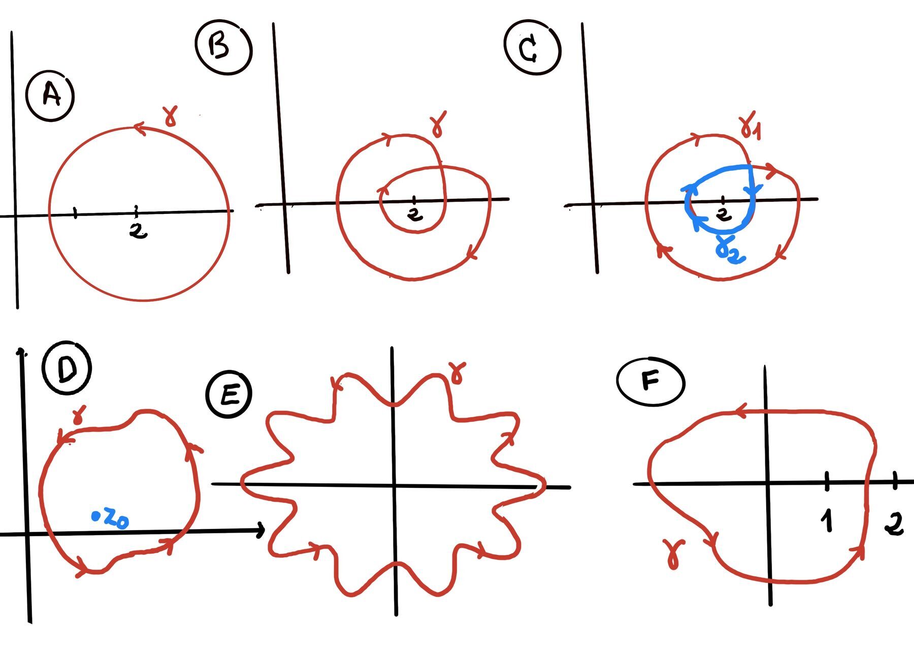
• Deformation of Contours. If two contours $\gamma_1$ and $\gamma_2 $ are homotopic (i.e., one can be continuously deformed into the other without crossing any singularities of f) in a domain where f(z) is analytic, then: $\int_{\gamma_1} f(z)dz = \int_{\gamma_2} f(z)dz.$

• Fundamental Theorem of Calculus for Contours. Suppose $\gamma$ is a contour (piecewise smooth path) from a to b, f is defined on a domain D containing $\gamma^*$ (the image of $\gamma$) and admits a primitive (antiderivative) F on D (i.e., $F'(z) = f(z)$), then $\int_{\gamma} f(z)dz = F(\gamma(b)) - F(\gamma(a))$. In particular, if $\gamma$ is a closed contour (i.e., $\gamma(a)=\gamma(b)$), this integral evaluates to zero, $\int_{\gamma} f(z)dz = 0.$

• Estimation Theorem or the Triangle Inequality for Integrals. The triangle inequality for integrals in complex analysis states thatfor any continuous complex function $f:[a,b] \to \mathbb{C}$ on a closed real interval [a,b] (f(t) = u(t) + iv(t), t a real parameter), the following holds: $∣\int_a^b f(t)dt| \leq \int_a^b |f(t)|dt$.

• Estimation Lemma (ML Inequality) for contour integrals. For any continuous complex function $f:[a,b] \to \mathbb{C}$ on a closed real interval [a,b] (f(z) = u(x, y) + iv(x, y)) with f bounded by some constant M along the entire contour, |f(z)| ≤ M for all $z \in \gamma^*$ (the image/trace of the contour in the complex plane), the following holds: $∣\int_\gamma f(z)dz| \leq M \cdot l(\gamma)$ where l(γ) is the arc length of the contour γ given by $\int_a^b |\gamma^{'}(t)|dt = \int_a^b \sqrt{x'(t)^2 + y'(t)^2}dt \text{ where } \gamma(t) = x(t) + iy(t)$.

Jordan’s curve theorem

In the plane, closed loops that don’t cross themselves behave like “boundaries.” Intuitively, drawing a circle on a sheet of paper divides the paper into two regions: the inside (a bounded region) and the outside (everything else). Jordan’s curve theorem makes this intuition precise — and shows that it holds not just for circles, but for any continuous loop that doesn’t cross itself, no matter how wild or irregular its shape.

This simple-looking fact is surprisingly deep. Although the statement is easy to believe for smooth curves like circles and ellipses, the theorem must also handle pathological cases: curves that are nowhere differentiable, curves with fractal-like boundaries, curves that oscillate infinitely. The full proof is non-trivial and constitutes a landmark result at the foundation of topology and complex analysis.

Definition. A simple closed curve (Jordan curve) is a continuous loop in the plane that does not intersect itself and starts and ends at the same point.

Formal definition. A map $\gamma:[a,b]\to\mathbb{R}^2$ (or ($\mathbb{C})$) is a simple closed curve if:

1. Closed: The curve starts and ends at the same point, $\gamma(a)=\gamma(b)$.
2. Simple, meaning $\gamma$ is injective on [a,b), $\gamma(t_1) = \gamma(t_2)$ with $t_1, t_2 \in [a, b)$ implies $t_1 = t_2$. The curve does not intersect itself anywhere except at its starting and ending points (which are the same).
3. Continuous: The curve is continuous, meaning it can be drawn without lifting the pencil from the paper.

Examples and non-examples (Figures 1 & 2)

Simple closed curves (Jordan curves):

• Circles: $\gamma(t) = \cos t + i\sin t$, $t \in [0, 2\pi]$.
• Ellipses: $\gamma(t) = a\cos t + ib\sin t$.
• Polygons: triangles, squares, any simple (non-self-intersecting) polygon.
• Irregular loops: any continuous closed curve that doesn’t cross itself, no matter how “wiggly.”

Not simple closed curves:

• Figure-eight: self-intersects at the crossing point.
• Open curves: line segments, rays, arcs — these fail the closedness condition.
• Curves that retrace themselves: e.g., $\gamma(t) = e^{it}$, $t \in [0, 4\pi]$ traverses the unit circle twice, so it is not injective on $[0, 4\pi)$.
• Curves with cusps that cross: any loop that touches or crosses itself at an interior point.

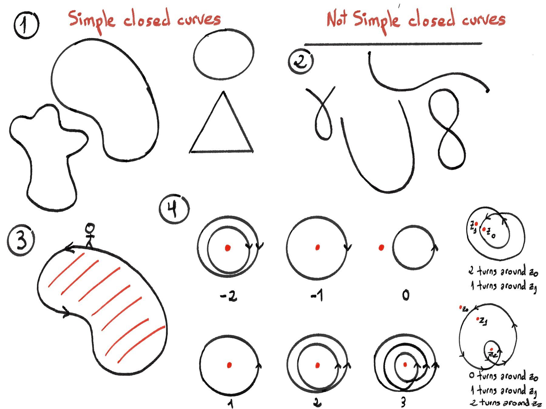Figure 1 (left block): examples of simple closed curves. Figure 2 (right block): not simple.

Definition. A region or set $U\subset\mathbb{C}$ is connected if any two points of U can be joined by a continuous path lying entirely in the region or set U.

A domain D is simply connected if it is connected and every closed loop in D can be continuously shrunk to a point inside D.

Jordan’s curve theorem. Any simple closed curve (a continuous loop in the plane that does not intersect itself) separates the plane into two components or disjoint connected regions: one interior (bounded) and one exterior (unbounded). The curve itself is the boundary of both regions. In other words, it partitions the plane into exactly three disjoint sets:

1. The Curve itself ($\gamma$) is the boundary between these two regions or components.
2. The Interior or inside ($\mathcal{Int}(\gamma), \mathcal{I}(\gamma)$) is the finite area enclosed by the curve (e.g., if you draw a circle on a piece of paper, the interior region would be everything inside the circle). It is a bounded, open, connected region inside of γ.
3. The Exterior or outside ($\mathcal{Ext}(\gamma), \mathcal{O}(\gamma)$) is the infinite area outside the curve (e.g., using the same circle example, the exterior region would include all points on the paper that are not inside the circle). It is an unbounded, open, connected region.

The Jordan’s curve theorem leads directly to several critical concepts:

1. Every path from inside to outside crosses the curve.
   If $p \in \operatorname{Int}(\gamma)$ and $q \in \operatorname{Ext}(\gamma)$, then any continuous path from $p$ to $q$ must intersect $\gamma^*$. This is because $\operatorname{Int}(\gamma)$ and $\operatorname{Ext}(\gamma)$ are distinct connected components of $\mathbb{R}^2 \setminus \gamma^*$: no continuous path can pass from one to the other without crossing the boundary.
2. The “Inside” and “Outside” are Well-Defined.
   For any Jordan curve, the concepts of “inside” and “outside” are mathematically rigorous and unambiguous, even for curves of extreme complexity. Every point lies either on the curve, strictly inside, or strictly outside.
3. The Complement is Disconnected.
   The plane minus the curve ($\mathbb{C}∖ \gamma$) is a disconnected space, with the interior and exterior being its two connected components, $\mathbb{C} \setminus \gamma^* = \operatorname{Int}(\gamma) \cup \operatorname{Ext}(\gamma),$ and this union is disjoint.
4. The Interior Is Simply Connected.
   The bounded component $\operatorname{Int}(\gamma)$ is simply connected — it has no “holes.” This is essential for complex analysis: Cauchy’s theorem applies to functions holomorphic on simply connected domains.
5. The Winding Number Is Well-Defined.
   It guarantees that the winding number $n(\gamma, z_0)$ is a powerful and well-defined tool for analyzing points relative to a curve.
   For a positively oriented Jordan curve: $n(\gamma, z_0) = \begin{cases} 1 & \text{if } z_0 \in \operatorname{Int}(\gamma), \\ 0 & \text{if } z_0 \in \operatorname{Ext}(\gamma). \end{cases}$

Examples

• The Unit Circle. Let $\gamma: [0, 2\pi] \to \mathbb{C}$ be defined as $\gamma(t) = \cos(t) + i\sin(t), 0 \le t \le 2\pi$. This parameterization describes the unit circle in the complex plane counterclockwise.

The interior of the curve, denoted as $\mathcal{Int}(\gamma)$, is given by $\mathcal{Int}(\gamma) = \{ z: |z| \lt 1 \}$— the open unit disk. which represents all complex numbers whose magnitudes are less than 1. Conversely, the exterior of the curve, denoted as $\mathcal{Ext}(\gamma)$, is defined as $\mathcal{Ext}(\gamma) = \{ z: |z| \gt 1 \}$ encompassing all complex numbers with magnitudes greater than 1.

Any path from $z=0$ (inside) to $z=2$ (outside) must cross the circle $|z|=1$. As $t$ increases, we move counter-clockwise. The interior (disk) stays to our left, so this is the positive orientation.

The three sets $\{|z| < 1\}$, $\{|z| = 1\}$, $\{|z| > 1\}$ partition $\mathbb{C}$. The interior is bounded and simply connected; the exterior is unbounded. The unit circle is the common boundary.

Orientation

The Jordan curve theorem tells us that the plane is divided into two regions, but to do contour integration, we also need to specify which direction we traverse the curve.

Definition. A simple closed contour γ is positively orientated (counterclockwise) if, as you traverse it, the bounded interior region (Int(γ)) is always to (stays on or appears to) your left (tracing the curve counterclockwise places the interior on the left). Conversely, it is negatively orientated if the interior is to your right (Figure 3).

Imagine walking along a circular path surrounding a beautiful garden. If you are walking counterclockwise and the garden (the interior) is on your left, you are positively oriented. If the garden is on your right, you are walking clockwise (negatively oriented).

Definition. For a positively oriented contour, the “inside” is the bounded component (Int(γ)). For a negatively oriented contour, the “inside” is the unbounded component (Ext(γ)).

However, in most practical applications, especially in complex analysis (e.g., Cauchy’s Integral Theorem), we standardize our curves to be positively oriented (counterclockwise). Therefore, unless stated otherwise, “the inside of a simple closed contour” universally refers to the bounded region.

Role in Complex Analysis

The Jordan curve theorem underpins virtually all of complex analysis involving contour integration:

Result	How Jordan’s theorem enables it
Cauchy’s theorem	Guarantees $\mathcal{Int}(\gamma)$ is a well-defined, bounded, simply connected domain where holomorphic functions have primitives
Cauchy integral formula	The formula requires $z_0$ to be “inside” $\gamma$ — Jordan’s theorem makes “inside” precise
Residue theorem	We must identify which singularities lie “inside” the contour
Winding number	Jordan’s theorem guarantees $n(\gamma, z_0) \in \{0, 1\}$ for Jordan curves, $1 \text{ if } z_0 \in \mathcal{Int}(\gamma)$
Maximum modulus principle	Applies on bounded domains; Jordan’s theorem ensures the interior is compact, hence bounded
Argument principle	Counting zeros and poles “inside” a contour requires a well-defined interior

The Jordan Curve Theorem is not merely a topological curiosity —it is the bedrock upon which the geometric intuitions of complex analysis rest. Every time we say “inside the contour,” “enclosed singularity,” or “simply connected domain,” we invoke Jordan’s result.