The Trace-Determinant Plane

Do, or do not. There is no try, Yoda.

The problem is not the problem. The problem is your attitude about the problem, Captain Jack Sparrow

The Trace-Determinant Plane

Understanding the behavior of linear systems of differential equations is essential in many disciplines like engineering, physics, and applied mathematics. One powerful tool for analyzing such systems, without having to solve them explicitly, is the Trace-Determinant (T-D) Plane, which helps us predict the nature of solutions and classify phase portraits instantly without solving the system explicitly.

Consider a two-linear system of differential equations: $(\begin{smallmatrix}x'\\\ y'\end{smallmatrix}) = (\begin{smallmatrix}a & b\\\ c & d\end{smallmatrix})(\begin{smallmatrix}x\\\ y\end{smallmatrix})$

This can be written in matrix form: $(\begin{smallmatrix}x'\\\ y'\end{smallmatrix}) = A(\begin{smallmatrix}x\\\ y\end{smallmatrix})$ where $A = (\begin{smallmatrix}a & b\\\ c & d\end{smallmatrix})$ is the coefficient 2 x 2 matrix.

Eigenvalues and Their Importance

To understand how the system behaves over time, we need to find its eigenvalues $\lambda$. These are special numbers that give us critical information about the system’s dynamics. They are solutions to the characteristic equation $\det(A - \lambda I) = 0$,, where I is the identity matrix.

Finding the eigenvalues allows us to:

1. Determine the types of equilibrium points (e.g., nodes, saddles, spirals, centers).
2. Understand whether solutions grow, decay, or oscillate.
3. Sketch the phase portrait, which shows the trajectories of solutions in the xy-plane.

A phase plane is a graphical representation of the system's solutions. Solutions to the system are plotted as curves in the phase plane called trajectories or orbits. Each point on a trajectory represents the state of the system at a particular time. Following the trajectory shows how the state of the system evolves over time (as $t \to \infty$.)

The characteristic polynomial is obtained from the determinant: $\det(A - \lambda I) = $.

For our 2 x 2 matrix, this becomes: $\det\begin{pmatrix} a-\lambda & b \\ c & d-\lambda \end{pmatrix} = (a-\lambda)(d-\lambda) - bc = 0$

Expanding and simplifying this expression yields: $\lambda^2 - (a+d)\lambda + (ad-bc) = 0$

We define two important quantities:

• Trace (T): The sum of the diagonal elements of the matrix A, so T = a + d.
• Determinant (D): The determinant of A, so D = det(A) = ad−bc.

Using these definitions, the characteristic polynomial simplifies beautifully to: $\lambda^2 - T\lambda + D = 0$

Theorem: If a $2 \times 2$ matrix $A$ has eigenvalues $\lambda_1$ and $\lambda_2$, then the trace of $A$ is their sum ($T = \lambda_1 + \lambda_2$) and the determinant is their product ($D = \lambda_1 \cdot \lambda_2$).

Classification via Trace and Determinant

Instead of explicitly computing the eigenvalues every time, we can use the trace and determinant to instantly understand the nature of the solutions. Thus, we can determine the phase portrait of a system $\vec{x}' = A\vec{x}$ by simply plotting the coordinate pair $(T, D)$ on a plane.

Using the quadratic formula on $\lambda^2 - T\lambda + D = 0$, the eigenvalues are given by: $\lambda = \frac{T \pm \sqrt{T^2 - 4D}}{2}$

We can see that the sign of the discriminant $\Delta = T^2 - 4D$ absolutely determines the nature of the eigenvalues of A (whether they are real, repeated, or complex).

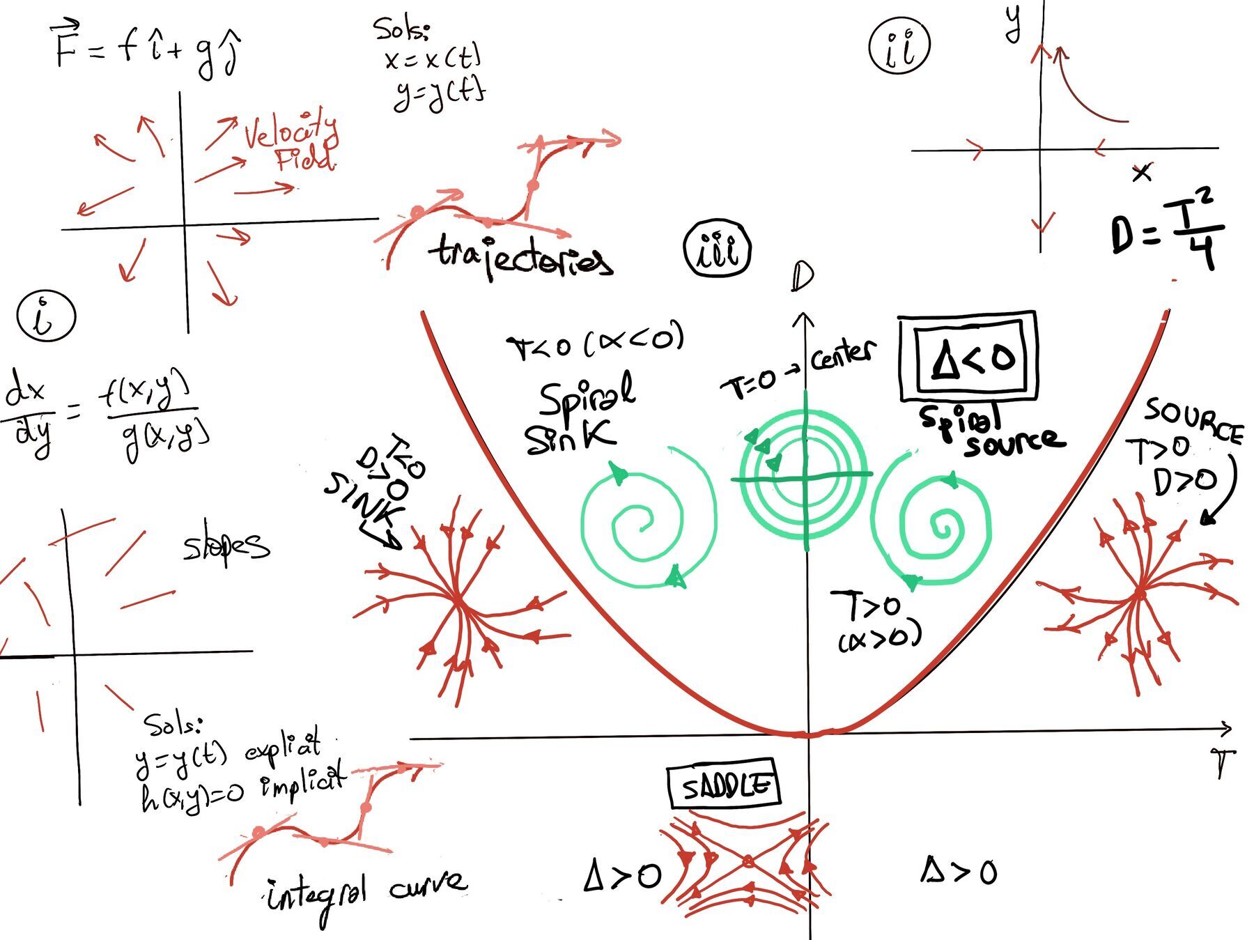
The Trace-Determinant Plane is a coordinate plane where the horizontal axis represents the Trace ($T$) and the vertical axis represents the Determinant ($D$). The parabola $D = \frac{T^2}{4}$ (which corresponds to $\Delta = 0$) acts as the primary boundary dividing the plane into distinct behavioral regions.

Regions in the T-D Plane

• Above the parabola $D > \frac{T^2}{4}$. Here, the discriminant $\Delta = T^2 - 4D < 0$. This corresponds to systems with complex conjugate eigenvalues $\lambda_{1,2} = \alpha \pm i\beta$. System Behavior: Spirals or Centers.

1. If $T > 0$ (Right side): The real part ($\frac{T}{2}$) is positive $\implies$ Unstable Spiral (Source).
2. If $T < 0$ (Left side): The real part is negative $\implies$ Stable Spiral (Sink).
3. If $T = 0$ (Exactly on the positive $D$-axis): Purely imaginary eigenvalues $\implies$ Center (Stable, periodic orbits).

• On the Parabola ($D = \frac{T^2}{4}$): Here, $\Delta = 0$. This corresponds to systems with repeated real eigenvalues. System Behavior: Improper or Degenerate Nodes.

1. If $T > 0$: Unstable improper node.
2. If $T < 0$: Stable improper node.

• Below the Parabola ($D < \frac{T^2}{4}$ but $D > 0$): Here, $\Delta > 0$ and $D > 0$. The eigenvalues are real, distinct, and have the same sign (because their product $D = \lambda_1\lambda_2$ is positive). It corresponds to systems with real and distinct eigenvalues of the same sign. System Behavior: Nodes.

1. If $T > 0$: Both eigenvalues are positive $\implies$ Unstable Node (Source).
2. If $T < 0$: Both eigenvalues are negative $\implies$ Stable Node (Sink).

• Below the Horizontal Axis ($D < 0$): Here, the determinant is negative. Since $D = \lambda_1\lambda_2 < 0$, the eigenvalues must be real and have opposite signs (one positive, one negative).
  This corresponds exclusively to a Saddle Point. Saddle points are always unstable.

Change of Coordinates and Similarity Transformations

When we talk about changing coordinates in the context of linear systems, we’re essentially performing a similarity transformation (or conjugation) on the system’s matrix. This involves choosing a new basis using an invertible matrix $P$ that transforms the original matrix $A$ into a new matrix $A'$: $A' = P^{-1}AP$

Despite this change of perspective, the fundamental geometric properties of the system remain completely unchanged, specifically the trace and determinant.

Theorem: The trace and determinant of a $2 \times 2$ matrix are invariant under a change of coordinates. Therefore, for any $2 \times 2$ matrix $A$ and any invertible $2 \times 2$ matrix $P$, the following hold true:

• $\det(P^{-1}AP) = \det(A)$
• $\text{tr}(P^{-1}AP) = \text{tr}(A)$

The determinant is a measure of how the matrix scales area (in 2D). When we change coordinates, we’re just looking at the same physical transformation from a different perspective (like tilting our head), so the underlying scaling factor (determinant) remains the same. The trace is the sum of the diagonal elements of a matrix. It is related to the sum of its eigenvalues. Since eigenvalues are intrinsic properties of the transformation (the fundamental “stretch factors”), they are indeed unaffected by the coordinate system, so the trace remains unchanged.

Corollary. The discriminant $\Delta = T^2 - 4D$ is invariant under a change of coordinates.

• Since both T and D are invariant, their combination $T^2 - 4D$ is mathematically guaranteed to be invariant.
• Because the discriminant is invariant, the fundamental nature of the eigenvalues (real, complex, repeated) and the qualitative behavior of the system (saddle, spiral, node) are universally preserved regardless of the coordinate system chosen.
• Universal Classification: We can classify all 2 × 2 linear systems purely based on their trace and determinant without worrying about the coordinate system.

Canonical Forms

Because similarity transformations preserve the system’s core behavior, we can safely ignore messy, complicated matrices and instead focus on simplified versions called canonical forms. Every $2 \times 2$ matrix can be transformed into one of these standard representations:

1. Complex Eigenvalues (Rotation + Scaling): $(\begin{smallmatrix}α & β\\\ -β & α\end{smallmatrix})$. Here, $\alpha$ and $\beta$ are real numbers. The eigenvalues are $\lambda = \alpha \pm i\beta$. This form clearly isolates the expansion/contraction ($\alpha$) from the rotation ($\beta$).
2. Distinct Real Eigenvalues (Diagonal Matrix): $$A' = \begin{pmatrix} \lambda_1 & 0 \\ 0 & \lambda_2 \end{pmatrix}$$ $\lambda_1$ and $\lambda_2$ are distinct real numbers. The matrix is perfectly diagonalizable, representing independent stretching along the $x$ and $y$ axes.
3. Repeated Real Eigenvalues (Scalar Matrix): $$A' = \begin{pmatrix} \lambda & 0 \\ 0 & \lambda \end{pmatrix}$$ $\lambda$ is a real number. This is a “star node” where the system stretches equally in every possible direction
4. Defective Matrix (Non-diagonalizable): $(\begin{smallmatrix}λ & 1\\\ 0 & λ\end{smallmatrix})$. This is the Jordan block form. The matrix is not diagonalizable due to a missing linearly independent eigenvector. Physically, this represents a system undergoing a sheer transformation alongside scaling.

Why Use Canonical Forms?

• Simplicity: They are the absolute simplest mathematical forms that capture the essence of each type of eigenvalue scenario.
• Easy to Analyze: It is trivial to compute eigenvalues, eigenvectors, matrix exponentials ($e^{At}$), and analytical solutions for these specific matrices.
• Representative: Any $2 \times 2$ linear system is essentially just one of these canonical forms viewed through a skewed coordinate grid.

Solving the Differential System

When a $2 \times 2$ matrix $A$ is diagonalizable, the general solution to the system $\vec{x}' = A\vec{x}$ is: $\vec{x}(t) = c_1 e^{\lambda_1 t}\vec{v_1} + c_2 e^{\lambda_2 t}\vec{v_2}$ where:

• $\lambda_1, \lambda_2$ are the eigenvalues of $A$.
• $\vec{v_1}, \vec{v_2}$ are the corresponding eigenvectors.
• $c_1, c_2$ are constants determined by the system’s initial conditions.

Types of Equilibrium Points

Depending on the nature of the eigenvalues, the equilibrium point at the origin $(0,0)$ can be classified into several distinct geometric categories:

1. Nodes (Real Eigenvalues, Same Sign)
   Stable Node: Both eigenvalues are real and negative ($\lambda_1, \lambda_2 < 0$). Trajectories approach the equilibrium along specific paths.
   Unstable Node: Both eigenvalues are real and positive ($\lambda_1, \lambda_2 > 0$). Trajectories move away from the equilibrium.
   Improper (Degenerate) Node: Repeated real eigenvalues. Depending on whether the matrix has a full set of eigenvectors (a “star” node) or is defective, trajectories either move radially or shear as they approach/recede.

2. Saddle Points (Real Eigenvalues, Opposite Signs)
   Eigenvalues are real with opposite signs ($\lambda_1 < 0 < \lambda_2$). Solutions approach the equilibrium along one eigenvector (the stable manifold) and depart along another eigenvector (the unstable manifold).

3. Spirals (Complex Eigenvalues, Non-zero Real Part)
   Stable Spiral: Real part is negative ($\alpha < 0$); solutions spiral inwards, decaying into the equilibrium.
   Unstable Spiral: Real part is positive ($\alpha > 0$); solutions spiral outwards, growing away from the equilibrium.

4. Centers (Purely Imaginary Eigenvalues)
   Eigenvalues are purely imaginary ($\alpha = 0$). Solutions form closed orbits (ellipses or circles). The system exhibits neutral stability, meaning trajectories neither converge to nor diverge from the origin.

Detailed Analysis of the Matrix with Complex Eigenvalues

To deeply understand complex eigenvalues, consider the canonical linear system $\vec{x}' = A\vec{x}$, where:$A = \begin{pmatrix} \alpha & \beta \\ -\beta & \alpha \end{pmatrix}$

To analyze the system, we find the eigenvalues of the matrix $A$ by solving the characteristic equation $\det(A - \lambda I) = 0$:

$\det\begin{pmatrix} \alpha-\lambda & \beta \\ -\beta & \alpha-\lambda \end{pmatrix} = (\alpha - \lambda)^2 - (-\beta)(\beta) = (\alpha - \lambda)^2 + \beta^2 = 0$

$(\alpha - \lambda)^2 = -\beta^2 \implies \alpha - \lambda = \pm i\beta$

Thus, the eigenvalues are complex conjugates: $\lambda = \alpha \pm i\beta$.

General Solution of the System

Theorem: Given a real $n \times n$ matrix $A$ with a complex eigenvalue $\lambda = \alpha + i\beta$ and a corresponding complex eigenvector $\vec{v}$, the general real solution to the system $\vec{x}' = A\vec{x}$ is: $x(t) = e^{αt}[C_1· Re(e^{iβt}\vec{v}) + C_2Im(e^{iβt}\vec{v})]$.

To apply this, we split the complex eigenvector into its real and imaginary parts: $\vec{v} = \vec{v_r} + i\vec{v_i}$. Using Euler’s formula ($e^{i\beta t} = \cos(\beta t) + i\sin(\beta t)$), we expand the core term: $e^{i\beta t}\vec{v} = (\cos(\beta t) + i\sin(\beta t))(\vec{v_r} + i\vec{v_i})$

$$= [\cos(\beta t)\vec{v_r} - \sin(\beta t)\vec{v_i}] + i[\cos(\beta t)\vec{v_i} + \sin(\beta t)\vec{v_r}]$$

This gives us two distinct, linearly independent real solutions:

• $\vec{x_r}(t) = \cos(\beta t)\vec{v_r} - \sin(\beta t)\vec{v_i}$
• $\vec{x_i}(t) = \cos(\beta t)\vec{v_i} + \sin(\beta t)\vec{v_r}$

Finding the Eigenvector

Let’s find the eigenvector for $\lambda = \alpha + i\beta$ by solving $(A - \lambda I)\vec{v} = \vec{0}$:

$$\begin{pmatrix} \alpha - (\alpha + i\beta) & \beta \\ -\beta & \alpha - (\alpha + i\beta) \end{pmatrix} \vec{v} = \begin{pmatrix} -i\beta & \beta \\ -\beta & -i\beta \end{pmatrix} \begin{pmatrix} a_1 \\ a_2 \end{pmatrix} = \begin{pmatrix} 0 \\ 0 \end{pmatrix}$$

Setting up the equation from the first row: $-i\beta a_1 + \beta a_2 = 0 \implies -i a_1 + a_2 = 0 \implies a_2 = i a_1$

If we choose $a_1 = 1$, then $a_2 = i$. Our complex eigenvector is: $\vec{v} = \begin{pmatrix} 1 \\ i \end{pmatrix} = \begin{pmatrix} 1 \\ 0 \end{pmatrix} + i\begin{pmatrix} 0 \\ 1 \end{pmatrix}$ where $\vec{v_r} = \begin{pmatrix} 1 \\ 0 \end{pmatrix}$ and $\vec{v_i} = \begin{pmatrix} 0 \\ 1 \end{pmatrix}$.

Constructing the Final Real Solution

Substitute $\vec{v_r}$ and $\vec{v_i}$ into our two real solution formulas:

• $\vec{x_r}(t) = \cos(\beta t)\begin{pmatrix} 1 \\ 0 \end{pmatrix} - \sin(\beta t)\begin{pmatrix} 0 \\ 1 \end{pmatrix} = \begin{pmatrix} \cos(\beta t) \\ -\sin(\beta t) \end{pmatrix}$
• $\vec{x_i}(t) = \cos(\beta t)\begin{pmatrix} 0 \\ 1 \end{pmatrix} + \sin(\beta t)\begin{pmatrix} 1 \\ 0 \end{pmatrix} = \begin{pmatrix} \sin(\beta t) \\ \cos(\beta t) \end{pmatrix}$

The general real solution to the system is the linear combination of these, scaled by the exponential envelope $e^{\alpha t}$: $\boxed{\vec{x}(t) = e^{\alpha t} \left[ C_1 \begin{pmatrix} \cos(\beta t) \\ -\sin(\beta t) \end{pmatrix} + C_2 \begin{pmatrix} \sin(\beta t) \\ \cos(\beta t) \end{pmatrix} \right]}$ where $C_1$ and $C_2$ are constants determined by initial conditions.

Breaking Down the Physics of the Solution:

• The Exponential Envelope ($e^{\alpha t}$):

1. $\alpha > 0$: The exponential term grows over time, pushing the amplitude of the solutions toward infinity.
2. $\alpha < 0$: The exponential term decays over time, dampening the solutions toward zero.
3. $\alpha = 0$: The exponential term is exactly $1$; solutions neither grow nor decay (sustained oscillation).

• The Trigonometric Functions ($\cos(\beta t), \sin(\beta t)$): These introduce continuous oscillations, causing the state vector to endlessly rotate around the origin. The parameter $\beta$ determines the frequency of this rotation.
• Visualization in Phase Space:

1. When $\alpha \neq 0$, the combination of rotation and exponential scaling creates trajectories that spiral either towards or away from the origin.
2. If $\alpha < 0$, the exponential decay causes trajectories to spiral inwards. The origin is a spiral sink (stable equilibrium).
3. If $\alpha > 0$, the exponential growth causes trajectories to spiral outward. The origin is a spiral source (unstable equilibrium).
4. When $\alpha = 0$, trajectories form perfectly closed orbits (loops). The origin is a center (neutrally stable).

Relationship Between Trace, Determinant, and Eigenvalues

We can confirm the behavior of this canonical matrix by relating it to the Trace ($T$) and Determinant ($D$). Recall that for any $2 \times 2$ matrix, the eigenvalues are given by $\lambda = \frac{T \pm \sqrt{T^2 - 4D}}{2}$.

For our matrix $A = \begin{pmatrix} \alpha & \beta \\ -\beta & \alpha \end{pmatrix}$:

• Trace (T): Sum of the diagonal elements (or sum of eigenvalues). $T = \alpha + \alpha = 2\alpha$
• Determinant (D): Product of the eigenvalues. $D = (\alpha)(\alpha) - (\beta)(-\beta) = \alpha^2 + \beta^2$
• Discriminant ($\Delta$): $\Delta = T^2 - 4D = (2\alpha)^2 - 4(\alpha^2 + \beta^2) = 4\alpha^2 - 4\alpha^2 - 4\beta^2 = -4\beta^2$

Since $\beta \neq 0$ (for purely complex roots) and $\beta^2 > 0$, the discriminant $\Delta = -4\beta^2$ is inherently strictly negative. This mathematically guarantees that the eigenvalues are complex conjugates, and the system exhibits oscillatory behavior.

Because the Real Part of the eigenvalues ($\alpha$) is directly proportional to the trace ($T = 2\alpha$), we can classify the system’s stability entirely by looking at the trace:

1. $T > 0$ ($\implies \alpha > 0$): The real part of the eigenvalues is positive. The system is unstable, and solutions spiral away from the origin. Origin is a Spiral Source.
2. $T < 0$ ($\implies \alpha < 0$): The real part of the eigenvalues is negative. The system is stable, and solutions spiral into the origin. Origin is a Spiral Sink.
3. $T = 0$ ($\implies \alpha = 0$): The real part of the eigenvalues is zero (purely imaginary). The system is neutrally stable; solutions neither grow nor decay. Origin is a Center.

Bibliography

1. NPTEL-NOC IITM, Introduction to Galois Theory.
2. Algebra, Second Edition, by Michael Artin.
3. LibreTexts, Calculus and Calculus 3e (Apex). Abstract and Geometric Algebra, Abstract Algebra: Theory and Applications (Judson).
4. Field and Galois Theory, by Patrick Morandi. Springer.
5. Michael Penn, and MathMajor.
6. Contemporary Abstract Algebra, Joseph, A. Gallian.
7. YouTube’s Andrew Misseldine: Calculus. College Algebra and Abstract Algebra.
8. MIT OpenCourseWare [18.03 Differential Equations, Spring 2006], YouTube by MIT OpenCourseWare.
9. Calculus Early Transcendentals: Differential & Multi-Variable Calculus for Social Sciences.