Heaviside Step Function and Time-Shifting Theorem

For instance, on the planet Earth, man had always assumed that he was more intelligent than dolphins because he had achieved so much—the wheel, New York, wars and so on—whilst all the dolphins had ever done was muck about in the water having a good time. But conversely, the dolphins had always believed that they were far more intelligent than man —for precisely the same reasons, Douglas Adams, The Hitchhiker’s Guide to the Galaxy.

Far out in the uncharted backwaters of the unfashionable end of the western spiral arm of the Galaxy lies a small unregarded yellow sun. Orbiting this at a distance of roughly ninety-two million miles is an utterly insignificant little blue green planet whose ape-descended life forms are so amazingly primitive that they still think digital watches are a pretty neat idea, Douglas Adams, The Hitchhiker’s Guide to the Galaxy.

Convolution: Definition and Basic Properties

Convolution is a powerful mathematical operation that blends two functions together to produce a third function. It is widely used in engineering, physics, signal processing, and applied mathematics to analyze systems and solve differential equations.

The convolution of two functions $f(t)$ and $g(t)$ is denoted by $(f * g)(t)$ and is defined by the integral $\boxed{(f * g)(t) = \int_{0}^{t} f(u)g(t-u) du}$

Properties of Convolution

1. Commutativity: $f * g = g * f$
2. Associativity: $f * (g * h) = (f * g) * h$. The convolution operation is associative, meaning that the order in which convolutions are performed does not affect the final result.
3. Distributivity Over Addition: $f * (g + h) = (f * g) + (f * h)$. Convolution distributes smoothly over addition.
4. Identity with the Delta Function: $f(t) * \delta(t) = f(t)$
   Convolving a function with the Dirac delta function returns the original function (much like multiplying by 1).
5. The Convolution Theorem: $\mathcal{L}(f(t)*g(t)) = \mathcal{L}(f(t))·\mathcal{L}(g(t))↭ \mathcal{L}^{-1}(F(s)·G(s)) = f(t)*g(t)$

Jump discontinuities and the Heaviside Step Function

In many physical applications (like flipping a switch in a circuit or applying a sudden mechanical force), we encounter functions that have sudden changes, known as jump discontinuities. A jump discontinuity occurs when a function abruptly jumps from one value to another at a specific point in time.

The most fundamental mathematical tool for modeling this is the Heaviside step function (also called the unit step function).

The unit step function, denoted as $u(t)$, is defined as having a value of zero for negative arguments and one for positive arguments. Mathematically, it is defined as:

$$u(t) = \begin{cases} 0, & t < 0 \\ \text{undefined (or } 0 \text{ or } 1), & t = 0 \\ 1, & t > 0 \end{cases}$$

Note on $t=0$: There is some ambiguity regarding the exact value of $u(0)$. Some textbooks define it as $0$, some as $1$, and others as $1/2$. For practical purposes involving integrals (like the Laplace Transform), this ambiguity is inconsequential for practical purposes. The area under a single point is zero, so the exact value at $t=0$ does not affect the calculation.

The Shifted Heaviside Step Function

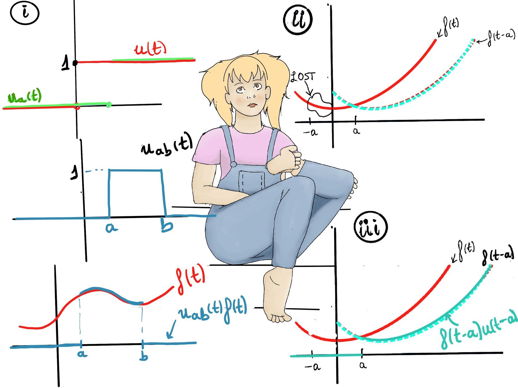
By shifting the unit step by a constant $a$, we create a new function that “activates” at $t = a$.

The shifted Heaviside step function is defined as:

$$u_a(t) = u(t - a) = \begin{cases} 0, & t < a \\ 1, & t \ge a \end{cases}$$

This shift allows us to control exactly when the jump occurs. Instead of jumping from $0$ to $1$ at $t = 0$, the function stays completely dormant until $t = a$, at which point it turns on. This is incredibly useful for modeling inputs or forces that start at a specific, delayed time.

The Unit Box Function (Windowing)

We can combine two shifted Heaviside functions to create a “box-shaped” function that is $1$ between two points ($a$ and $b$), and $0$ everywhere else. This is called the unit box function, denoted by $u_{ab}(t)$.

It is constructed by taking a step function that turns on at $t=a$, and subtracting a step function that turns on at $t=b$: $u_{ab}(t) = u(t-a) - u(t-b)$

$$u_{ab}(t) = \begin{cases} 0, & t < a \\ 1, & a \le t < b \\ 0, & t \ge b \end{cases}$$

When we multiply an arbitrary continuous function $f(t)$ by this unit box function, $f(t)u_{ab}(t)$. The function “turns on” 🔦 at t = a and “turns off” at t = b, we effectively “window” the function.

• For $t$ between $a$ and $b$, the function is multiplied by $1$, leaving it unchanged.
• For $t$ outside this interval, the function is multiplied by $0$, completely wiping it out.

$$f(t)u_{ab}(t) = \begin{cases} 0, & t < a \\ f(t), & a \le t < b \\ 0, & t \ge b \end{cases}$$

Laplace Transform of the Heaviside Step Function

Let’s calculate the standard Laplace transform of the basic unit step function $u(t)$: $\mathcal{L}\{u(t)\} = \int_{0}^{\infty} e^{-st}u(t) dt$

Since $u(t) = 1$ for all positive values of $t$, the integral simplifies exactly to the Laplace Transform of the constant $1$: $\mathcal{L}\{u(t)\} = \int_{0}^{\infty} e^{-st}(1) dt = \frac{1}{s}, \quad s > 0$, which is consistent with the Laplace Transform of the constant function 1 for s > 0.

Ensuring Uniqueness in the Inverse Transform

If we know that $\mathcal{L}\{1\} = \frac{1}{s}$ and $\mathcal{L}\{u(t)\} = \frac{1}{s}$, what is $\mathcal{L}^{-1}\left\{\frac{1}{s}\right\}$?

Because the standard Laplace transform only integrates from $t=0$ to infinity, it has “amnesia” regarding anything that happens before $t=0$ (the Laplace transform is only concerned with what happens for t ≥ 0). Therefore, any function that matches $f(t)$ for $t > 0$ will yield the exact same Laplace transform, regardless of its behavior in negative time.

To ensure uniqueness when taking the inverse transform, the mathematical community uses a strict convention: we assume all functions are exactly $0$ for $t < 0$.

Suppose that the Laplace Transform of f is F, $f(t)\leadsto F(s)$, the inverse Laplace transform of F(s) is f(t). We enforce this convention algebraically by multiplying the inverse transform by $u(t)$: $\boxed{\mathcal{L}^{-1}\{F(s)\} = f(t)u(t)}$

By applying the step function, we chop off any hypothetical “negative tail (we effectively cut off any behavior of f(t) for t < 0),” ensuring the inverse transform is well-defined and unique.

The T-Axis Translation Formula (Time-Shifting Theorem)

There is no direct formula for $\mathcal{L}\{f(t-a)\}$ without additional considerations. If you simply shift a function right by $a$, the Laplace integral still starts at $t=0$. This means it would require information about $f(t)$ for negative values (between $-a$ and $0$), which the Laplace transform inherently ignores.

To fix this, we ensure the shifted function only “begins” at $t=a$ by multiplying it by $u(t-a)$ (we basically address this issue by wiping out this area). If the original function starts at t = 0, the shifted function starts at t = a. The Heaviside function u(t − a) takes care of this, making the function zero for t < a and nonzero for t ≥ a. In other words, we can get a formula from the function u(t-a)·f(t-a).

In the context of the Laplace Transform, the T-axis translation formula deals with shifting a function in time. When you shift a function f(t) by a constant a (i.e., replace t with t −a), the Laplace Transform of the shifted function is related to the Laplace Transform of the original function through multiplication by an exponential factor. More formally, $u(t-a)f(t-a) \leadsto e^{-as}F(s)↭ \mathcal{L}(u(t-a)f(t-a)) = e^{-as}F(s)$ or equivalently $u(t-a)f(t) [\text{Observe t = (t +a) -a}] \leadsto e^{-as} \mathcal{L}(f(t+a)) = e^{-as}F(s+a)$ where:

• u(t -a) is the Heaviside step function, ensuring that the function is zero before t = a.
• f(t −a) is the original function, shifted by a.
• F(s) is the Laplace Transform of f(t), i.e., $F(s)=\mathcal{L}(f(t)).$ Refer to Figure iii for a visual representation and aid in understanding it.

Proof

We aim to prove that $\mathcal{L}\{u(t-a)f(t-a)\} = e^{-as}F(s)$.

By definition: $\mathcal{L}\{u(t-a)f(t-a)\} = \int_{0}^{\infty} e^{-st}u(t-a)f(t-a) dt$

Since $u(t-a) = 0$ for all $t < a$, the integral from $0$ to $a$ is zero. We can simply adjust our lower limit of integration to $a$, at which point $u(t-a)$ becomes $1$: $= \int_{a}^{\infty} e^{-st}f(t-a) dt$

Now, we perform a substitution (change of variables) to shift the integral back to $0$. Let $\tau = t - a$.

• This implies $t = \tau + a$ and $dt = d\tau$.
• Limits of integration. When $t = a$, $\tau = 0$. When $t \to \infty$, $\tau \to \infty$.

Substitute these into the integral: $= \int_{0}^{\infty} e^{-s(\tau+a)}f(\tau) d\tau = \int_{0}^{\infty} e^{-s\tau}e^{-sa}f(\tau) d\tau$

Since $e^{-sa}$ is a constant with respect to $\tau$, we can pull it out of the integral: $= e^{-as} \int_{0}^{\infty} e^{-s\tau}f(\tau) d\tau$

The remaining integral is exactly the definition of the standard Laplace Transform of $f(t)$! $\mathcal{L}\{u(t-a)f(t-a)\} =[\cdots] e^{-as}F(s)$ (Q.E.D)

$u(t-a)f(t-a) \leadsto e^{-as}\mathcal{L}(f(t)) = e^{-as}F(s) ↭ u(t-a)f(t-a) \leadsto e^{-as}\mathcal{L}(f(t))$

Similarly, $u(t-a)f(t+a-a) \leadsto e^{-as}\mathcal{L}(f(t+a))↭ u(t-a)f(t) \leadsto e^{-as}\mathcal{L}(f(t+a))$

Solved Laplace Transform Exercises

Exercise 1: The Laplace Transform of the Unit Box Function

The unit box function $u_{ab}(t)$ is a piecewise function that is $1$ within the interval $[a, b]$ and $0$ everywhere else (where $a$ and $b$ are constants with $a < b$).

It can be constructed using the Heaviside Step Function $u(t)$ by subtracting a step function that starts at $b$ from a step function that starts at $a$: $u_{ab}(t) = u(t - a) - u(t - b)$

Mathematically, it is defined as: $u_{ab}(t) = \begin{cases} 0, & t < a \\ 1, & a \le t < b \\ 0, & t \ge b \end{cases}$

Solution:

Recall the fundamental Laplace Transform of a shifted step function: $\mathcal{L}\{u(t - a)\} = \frac{e^{-as}}{s}$

Using the linearity property of the Laplace Transform, we can take the transform of each term separately: $\mathcal{L}\{u_{ab}(t)\} = \mathcal{L}\{u(t - a)\} - \mathcal{L}\{u(t - b)\} = \frac{e^{-as}}{s} - \frac{e^{-bs}}{s} =[\text{Simplify}] \frac{e^{-as} - e^{-bs}}{s}$

Key Insight: The Laplace Transform perfectly captures the unit box function’s behavior. The exponential terms explicitly define (or correspond to) the activation time ($e^{-as}$) and the deactivation time ($e^{-bs}$) of the signal.

Exercise 2: Laplace Transform of Shifted Polynomial Functions

Compute the Laplace Transform of the function: $f(t) = u(t - 1)t^2$

Solution:

1. Recall relevant Laplace Transform Properties.
   Time-Shifting Theorem (Alternative Form): $\mathcal{L}\{u(t - a)f(t)\} = e^{-as}\mathcal{L}\{f(t + a)\}$
   Laplace Transform of Polynomials: $\mathcal{L}\{t^n\} = \frac{n!}{s^{n+1}}$
2. Identify the parameters from our given function: $a = 1$ and $f(t) = t^2$
3. Apply the shifting theorem formula: $\mathcal{L}\{u(t - 1)t^2\} = e^{-1 \cdot s}\mathcal{L}\{(t + 1)^2\}$
4. Before transforming, expand the polynomial inside the Laplace operator: $(t + 1)^2 = t^2 + 2t + 1$
5. Using Laplace Transform of Polynomials: $\mathcal{L}\{u(t - 1)t^2\} = e^{-s}\mathcal{L}\{t^2 + 2t + 1\} = e^{-s}\left(\frac{2}{s^3} + \frac{2}{s^2} + \frac{1}{s}\right)$

Exercise 3: Inverse Laplace Transform using Convolution

Evaluate: $\mathcal{L}^{-1}\left\{\frac{1}{s^2 + 1} \cdot \frac{1}{s^2 + 1}\right\}$

Relevant Properties:
Convolution Theorem: $\mathcal{L}^{-1}\{F(s) \cdot G(s)\} = (f * g)(t) = \int_{0}^{t} f(\tau)g(t - \tau) d\tau$
Standard Transform: $\mathcal{L}^{-1}\left\{\frac{1}{s^2 + 1}\right\} = \sin(t)$

Solution:

1. Since both functions are $\sin(t)$, we need to calculate the following convolution: $\mathcal{L}^{-1}\left\{\frac{1}{s^2 + 1} \cdot \frac{1}{s^2 + 1}\right\} = \int_{0}^{t} \sin(\tau)\sin(t - \tau) d\tau$

2. To evaluate this integral, apply the trigonometric product-to-sum identity: $\sin(A)\sin(B) = \frac{1}{2}[\cos(A - B) - \cos(A + B)]$ where $A = \tau$ and $B = t - \tau$: $A - B = \tau - (t - \tau) = 2\tau - t$, $A + B = \tau + (t - \tau) = t$

3. Substitute this back into the integral: $= \frac{1}{2}\int_{0}^{t} [\cos(2\tau - t) - \cos(t)] d\tau$

4. Separate this into two distinct integrals with respect to $\tau$:
   First Integral: $\frac{1}{2}\int_{0}^{t} \cos(2\tau - t) d\tau$
   $\frac{1}{2}\int_{0}^{t} cos(2τ-t)dτ =[\text{Using the substitution u=2τ-t, du = 2dτ. When τ = 0, u = -t, When τ = t, u = t}] \frac{1}{2}\frac{1}{2}\int_{-t}^{t}cos(u)du = \frac{1}{4}sin(t)\bigg|_{-t}^{t} = \frac{1}{4}(sin(t)-sin(-t)) = \frac{1}{4}(sin(t)+sin(t)) = \frac{1}{2}sin(t)$
   Second Integral: $-\frac{1}{2}\int_{0}^{t} \cos(t) d\tau$
   Since $\cos(t)$ is a constant with respect to $\tau$, simply pull it out: $-\frac{1}{2}\cos(t) \int_{0}^{t} 1 d\tau = -\frac{1}{2}t\cos(t)$

5. Finally, combine the results, and we get: $\mathcal{L}^{-1}\left\{\frac{1}{s^2 + 1} \cdot \frac{1}{s^2 + 1}\right\} = \frac{1}{2}\sin(t) - \frac{1}{2}t\cos(t)$

Exercise 4: Inverse Transform with an Exponential Term

Evaluate: $\mathcal{L}^{-1}\left\{\frac{1 + e^{-\pi s}}{s^2 + 1}\right\}$

Relevant Properties:
First Shifting Theorem (Inverse): $\mathcal{L}^{-1}\{e^{-as}F(s)\} = u(t - a)f(t - a)$ Standard Transform: $\mathcal{L}^{-1}\left\{\frac{1}{s^2 + 1}\right\} = \sin(t)$

Solution:

1. Decompose the fraction.
   Break the expression into two simpler terms so we can evaluate them individually: $Y(s) = \frac{1}{s^2 + 1} + \frac{e^{-\pi s}}{s^2 + 1}$

2. Compute the Inverse Laplace Transform of Each Term.
   Term 1: $\mathcal{L}^{-1}\left\{\frac{1}{s^2 + 1}\right\} = u(t)\sin(t)$ for $t \ge 0$. The reason that we need to add the step function is because of the presence of exponential in the original formula.
   Term 2: Using the shifting theorem where $a = \pi$ and $f(t) = \sin(t)$: $\mathcal{L}^{-1}\left\{\frac{e^{-\pi s}}{s^2 + 1}\right\} = u(t - \pi)\sin(t - \pi)$

3. Combine the Results. $f(t) = u(t)\sin(t) + u(t - \pi)\sin(t - \pi)$

4. Simplify the Piecewise Function.
   Let’s evaluate what this function actually looks like in different time domains.
   For $0 \le t < \pi$, the second term hasn’t activated yet: $f(t) = \sin(t)$
   For $t \ge \pi$, both terms are active. Recall the trigonometric shift identity $\sin(t - \pi) = -\sin(t)$: $f(t) = \sin(t) + \sin(t - \pi) = \sin(t) - \sin(t) = 0$.
   Putting it all together:
   

   $$f(t) = \begin{cases} \sin(t), & 0 \le t < \pi \\ 0, & t \ge \pi \end{cases}$$

Key Insight: This creates a single, isolated “pulse”. The sine wave starts at $t=0$, but exactly half a wavelength later at $t=\pi$, the exponential shift effectively creates an inverted sine wave that perfectly cancels out the original, “turning off” the signal entirely.

Bibliography

1. NPTEL-NOC IITM, Introduction to Galois Theory.
2. Algebra, Second Edition, by Michael Artin.
3. LibreTexts, Calculus and Calculus 3e (Apex). Abstract and Geometric Algebra, Abstract Algebra: Theory and Applications (Judson).
4. Field and Galois Theory, by Patrick Morandi. Springer.
5. Michael Penn, and MathMajor.
6. Contemporary Abstract Algebra, Joseph, A. Gallian.
7. YouTube’s Andrew Misseldine: Calculus. College Algebra and Abstract Algebra.
8. MIT OpenCourseWare [18.03 Differential Equations, Spring 2006], YouTube by MIT OpenCourseWare.
9. Calculus Early Transcendentals: Differential & Multi-Variable Calculus for Social Sciences.