Solving Linear ODEs using the Laplace Transform. Worked Examples

Life is a math equation. In order to gain the most, you have to know how to convert negatives into positives, Anonymous

Laplace Transform

The Laplace Transform of a function f(t), where t ≥ 0, is defined as $\mathcal{L}(f(t)) = \int_{0}^{∞} f(t)e^{-st}dt = F(s)$.

One of the most important properties of the Laplace Transform is linearity, which states: $\mathcal{L}(af(t)+bg(t)) = a\mathcal{L}(f(t))+b\mathcal{L}(g(t))$

Table of Common Laplace Transforms

The following table summarizes the most frequent mappings used in system analysis.

Function	Laplace Transform
Unit Step, u(t)	$\mathcal{L}(u(t)) = \frac{1}{s}, s > 0$
Exponential, $e^{at}$	$\frac{1}{s - a}, s > a$
Complex Exp $e^{(a + bi)t}$	$\mathcal{L}(e^{(a + bi)t}) = \frac{1}{s - (a + bi)}, s > a$
Cosine $\cos(\omega t)$	$\mathcal{L}(\cos(\omega t)) = \frac{s}{s^2 + \omega^2}, s > 0$
Sine $\sin(\omega t)$	$\mathcal{L}(\sin(\omega t)) = \frac{\omega}{s^2 + \omega^2}, s > 0$
Power, $t^n$	$\mathcal{L}(t^n) = \frac{n!}{s^{n+1}}, s > 0$
Delayed Step, $u(t-a)$	$\mathcal{L}(u(t-a)) = \frac{e^{-as}}{s}, s > 0$
Dirac Delta $\delta(t-a)$	$\mathcal{L}(\delta(t-a)) = e^{-as}, a \geq 0$
$\frac{1}{t}$	$\mathcal{L}\left(\frac{1}{t}\right) = \text{not defined}$
$e^{-bt} \cos(\omega t)$	$\mathcal{L}(e^{-bt} \cos(\omega t)) = \frac{s + b}{(s + b)^2 + \omega^2}, s > -b$
$e^{-bt} \sin(\omega t)$	$\mathcal{L}(e^{-bt} \sin(\omega t)) = \frac{\omega}{(s + b)^2 + \omega^2}, s > -b$
$e^{at}f(t)$	$\mathcal{L}(e^{at}f(t)) = F(s-a)$

Solving Linear ODEs using the Laplace Transform: Worked Examples

Problem 1: Overdamped System

Solve: $y'' - 3y' + 2y = 0$. Initial Conditions: $y(0) = 1, \ y'(0) = 0$

Step 1 👣: Take the Laplace Transform of Both Side

Apply the transform linearly across the equation: $\mathcal{L}\{y''\} - 3\mathcal{L}\{y'\} + 2\mathcal{L}\{y\} = 0$

Step 2 👣: Substitute Transforms of the derivatives and Initial Conditions.

Recall the derivative rules: $(s^2Y(s) - sy(0) - y'(0)) - 3(sY(s) - y(0)) + 2Y(s) = 0$.

Substitute $y(0) = 1$ and $y'(0) = 0$: $(s^2Y(s) - s \cdot 1 - 0) - 3(sY(s) - 1) + 2Y(s) = 0$

Simplify, $s^2Y(s) - s - 3sY(s) + 3 + 2Y(s) = 0$

Group the $Y(s)$ terms together and move the rest to the right side: $(s^2 - 3s + 2)Y(s) = s - 3$

Step 3 👣: Solve for $Y(s)$

$$Y(s) = \frac{s - 3}{s^2 - 3s + 2}$$

Factor the denominator to prepare for partial fractions: $Y(s) = \frac{s - 3}{(s - 1)(s - 2)}$

Step 4 👣: Partial Fraction Decomposition

$$\frac{s - 3}{(s - 1)(s - 2)} = \frac{A}{s - 1} + \frac{B}{s - 2}$$

Multiply by the common denominator: $s - 3 = A(s - 2) + B(s - 1)$

Tip: Use the “cover-up” (or root substitution) method here for speed!

• Let $s = 1 \implies -2 = A(-1) \implies A = 2$
• Let $s = 2 \implies -1 = B(1) \implies B = -1$

Therefore, $Y(s) = \frac{2}{s - 1} - \frac{1}{s - 2}$

Step 5 👣: Apply the Inverse Laplace Transform

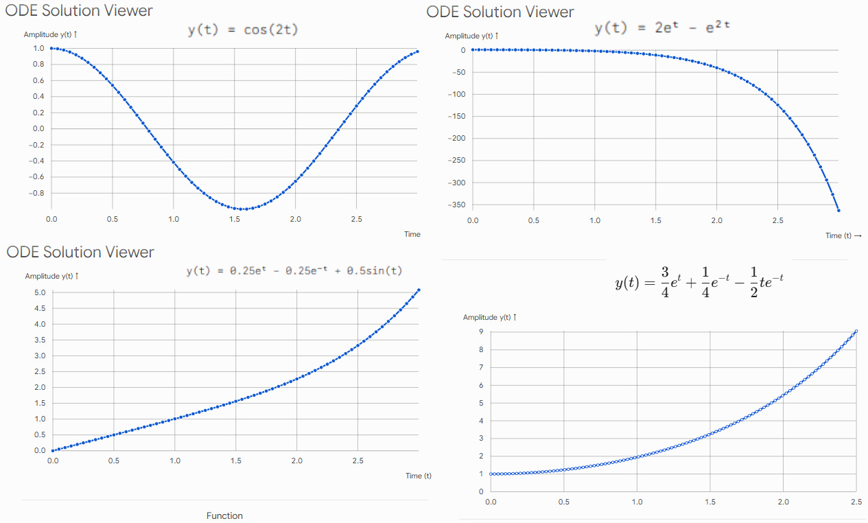
Using the standard transform $\mathcal{L}^{-1}\left\{\frac{1}{s-a}\right\} = e^{at}$, we get: $\boxed{y(t) = 2e^t - e^{2t}}$

Problem 2: Simple Harmonic Oscillator

Solve: $y'' + 4y = 0$. Initial Conditions: $y(0) = 1, \ y'(0) = 0$

Step 1 👣: Take the Laplace Transform of Both Sides

$$\mathcal{L}\{y''\} + 4\mathcal{L}\{y\} = 0$$

Step 2 👣: Substitute Transforms and Initial Conditions

Using the transforms of the derivatives: $(s^2Y(s) - sy(0) - y'(0)) + 4Y(s) = 0$

Substitute $y(0) = 1, \ y'(0) = 0$, $(s^2Y(s) - s \cdot 1 - 0) + 4Y(s) = 0$

Group the terms: $(s^2 + 4)Y(s) = s$

Step 3 👣: Solve for $Y(s)$

$$Y(s) = \frac{s}{s^2 + 4}$$

Step 4 👣: Apply the Inverse Laplace Transform

Looking at our standard tables, this perfectly matches the cosine transform formula $\mathcal{L}^{-1}\left\{\frac{s}{s^2+a^2}\right\} = \cos(at)$. Here, $a^2 = 4 \implies a = 2$.

Therefore, $\boxed{y(t) = \cos(2t)}$. This equation perfectly models an undamped mass on a spring released from $y=1$ with no initial velocity.

Problem 3: 4th-Order Differential Equation

Solve: $y^{(4)} - y = 0$. Initial Conditions: $y(0) = 0, \ y'(0) = 1, \ y''(0) = 0, \ y'''(0) = 0$

Step 1 👣: Take the Laplace Transform of Both Sides

$$\mathcal{L}\{y^{(4)}\} - \mathcal{L}\{y\} = 0$$

Step 2 👣: Substitute Transforms and Initial Conditions

The 4th derivative expands to: $\left(s^4Y(s) - s^3y(0) - s^2y'(0) - sy''(0) - y'''(0)\right) - Y(s) = 0$

Substitute the initial conditions (most of them are zero!): $(s^4Y(s) - 0 - s^2(1) - 0 - 0) - Y(s) = 0$

Simplify, $s^4Y(s) - s^2 - Y(s) = 0$

Group the terms: $Y(s)(s^4 - 1) = s^2$

Step 3 👣: Solve for $Y(s)$

$$Y(s) = \frac{s^2}{s^4 - 1}$$

Step 4 👣: Partial Fraction Decomposition

First, fully factor the denominator using the difference of squares: $s^4 - 1 = (s^2 - 1)(s^2 + 1) = (s - 1)(s + 1)(s^2 + 1)$.

Therefore, $\frac{s^2}{(s - 1)(s + 1)(s^2 + 1)} = \frac{A}{s - 1} + \frac{B}{s + 1} + \frac{Cs + D}{s^2 + 1}$

Multiply by the common denominator: $s^2 = A(s + 1)(s^2 + 1) + B(s - 1)(s^2 + 1) + (Cs + D)(s - 1)(s + 1)$

Let’s solve for the constants:

• Evaluate at $s = 1 \implies 1 = A(2)(2) \implies 4A = 1 \implies A = \frac{1}{4}$
• Evaluate at $s = -1 \implies 1 = B(-2)(2) \implies -4B = 1 \implies B = -\frac{1}{4}$
• Evaluate at $s = 0 \implies 0 = A(1)(1) + B(-1)(1) + D(-1) \implies 0 = \frac{1}{4} + \frac{1}{4} - D \implies D = \frac{1}{2}$
• Evaluate at $s = 2 \implies 4 = A(3)(5) + B(1)(5) + (2C + D)(1)(3)$
  $4 = 15\left(\frac{1}{4}\right) + 5\left(-\frac{1}{4}\right) + 3\left(2C + \frac{1}{2}\right)$
  $4 = \frac{10}{4} + 6C + \frac{3}{2} \implies 4 = \frac{5}{2} + \frac{3}{2} + 6C \implies 4 = 4 + 6C \implies C = 0$

So, our decomposed function is: $Y(s) = \frac{1/4}{s - 1} - \frac{1/4}{s + 1} + \frac{1/2}{s^2 + 1}$

Step 5 👣: Apply the Inverse Laplace Transform

Using our tables for exponentials and sine ($\mathcal{L}^{-1}\left\{\frac{a}{s^2+a^2}\right\} = \sin(at)$): $\boxed{y(t) = \frac{1}{4}e^t - \frac{1}{4}e^{-t} + \frac{1}{2}\sin(t)}$

We can rewrite the first two terms using hyperbolic functions! Since $\sinh(t) = \frac{e^t - e^{-t}}{2}$, your answer can be elegantly written as: $\boxed{y(t) = \frac{1}{2}\sinh(t) + \frac{1}{2}\sin(t)}$

Observe below the ODE solutions we’ve just derived and their distinct physical behaviors:

1. $y(t) = 2e^{t} - e^{2t}$, for large t, the $e^{2t}$ term dominates, so $y(t) \sim -e^{2t} \quad (t \to \infty)$, which actually means runaway exponential blow-up to $-\infty$.
2. $y(t) = \cos(2t)$, pure (stable) oscillation with constant amplitude 1. No growth, no decay.
3. $y(t) \frac{1}{4}e^t - \frac{1}{4}e^{-t} + \frac{1}{2}\sin t$. As $t \to \infty: y(t) \sim \frac{1}{4}e^t,$ because $e^t$ dominates both the bounded oscillation $\sin t$ and the vanishing exponential $e^{-t}$. So the exponential growth completely outmatches the sinusoidal term: the oscillation becomes a tiny ripple riding on a rapidly growing curve.

Bibliography

1. NPTEL-NOC IITM, Introduction to Galois Theory.
2. Algebra, Second Edition, by Michael Artin.
3. LibreTexts, Calculus and Calculus 3e (Apex). Abstract and Geometric Algebra, Abstract Algebra: Theory and Applications (Judson).
4. Field and Galois Theory, by Patrick Morandi. Springer.
5. Michael Penn, and MathMajor.
6. Contemporary Abstract Algebra, Joseph, A. Gallian.
7. YouTube’s Andrew Misseldine: Calculus. College Algebra and Abstract Algebra.
8. MIT OpenCourseWare [18.03 Differential Equations, Spring 2006], YouTube by MIT OpenCourseWare.
9. Calculus Early Transcendentals: Differential & Multi-Variable Calculus for Social Sciences.