Solving Linear ODE's using the Laplace Theorem

Monsters exist, but they are too few in number to be truly dangerous. More dangerous are the common men, the functionaries ready to believe and to act without asking questions, Primo Levi

Laplace Transform

The Laplace Transform of a function f(t), where t ≥ 0, is defined as $\mathcal{L}(f(t)) = \int_{0}^{∞} f(t)e^{-st}dt = F(s)$.

One of the most important properties of the Laplace Transform is linearity, which states: $\mathcal{L}(af(t)+bg(t)) = a\mathcal{L}(f(t))+b\mathcal{L}(g(t))$

Table of Common Laplace Transforms

The following table summarizes the most frequent mappings used in system analysis.

Solving Linear ODEs using the Laplace Transform

The Laplace Transform is one of the most powerful mathematical tools for solving linear ordinary differential equations (ODEs), particularly those with constant coefficients and specific Initial Value Problems (IVPs).

💡 The Core Concept. By transforming differential equations from the time domain ($t$) into algebraic equations in the complex frequency domain ($s$), we simplify the process of finding solutions to these equations. This method is particularly useful because it converts differential equations, which involve derivatives, into algebraic equations, which are generally easier to solve.

The Initial Value Problem (IVP)

Consider the following second-order linear ODE with constant coefficients: $y'' + Ay' + By = h(t)$ where:

• y(t) is the unknown function of time we want to solve for (the system’s response).
• A and B are constants (representing physical properties like damping and stiffness).
• $h(t)$ is a given forcing function (the external input to the system). If $h(t) = 0$, the equation is homogeneous.
• The initial conditions are defined at $t=0$: $y(0) = y_0$ and $y'(0) = y'_0$.

Applying the Laplace Transform

Our goal is to solve this equation for y(t) using the Laplace Transform. The key idea is that the Laplace Transform converts the time-domain differential equation into an algebraic equation in the complex frequency variable s. This transformation simplifies solving the differential equation by turning it into an algebraic problem.

To map this problem into the $s$-domain, we apply the Laplace operator $\mathcal{L}\{\}$ to both sides. First, recall how the transform handles derivatives:

• Laplace Transform of a function y(t): $\mathcal{L}(y(t)) = \int_{0}^{∞} e^{-st}y(t)dt = Y(s)$
• Laplace Transform of the first derivative y′(t): $\mathcal{L}(y'(t)) = sY(s) -y(0) = sY(s) -y_0$
• Laplace Transform of the first derivative y’′(t): $\mathcal{L}(y'(t)) = s^2Y(s) -sy(0) -y'(0) = s^2Y(s) -sy_0 -y'_0.$

These formulas are derived using integration by parts and incorporate the initial conditions.

Transforming the Differential Equation

By the property of linearity, we can apply the transform to each term individually: $\mathcal{L}\{y''\} + A\mathcal{L}\{y'\} + B\mathcal{L}\{y\} = \mathcal{L}\{h(t)\}$

Substitute the derivative expansions into the equation: $(s^2Y(s) - sy_0 - y'_0) + A(sY(s) - y_0) + BY(s) = H(s)$ where $H(s) = \mathcal{L}\{h(t)\}$

Next, factor out $Y(s)$ and group all the initial condition terms on the other side: $Y(s)(s^2 + As + B) = H(s) + sy_0 + y'_0 + Ay_0$

The polynomial $(s^2 + As + B)$ is known as the characteristic polynomial of the system. Finally, isolate $Y(s)$: $\boxed{Y(s) = \frac{H(s) + sy_0 + y'_0 + Ay_0}{s^2 + As + B}}$

This equation represents the solution in the frequency domain, represented as Y(s), an algebraic expression in terms of s. Typically, the result is a rational function $\frac{p(s)}{q(s)}$, where p(s) and q(s) are polynomials in S.

Finding the Time-Domain Solution y(t)

To find the solution $y(t)$ in the time domain (our final answer), we must reverse the process by applying the Inverse Laplace Transform: $y(t) = \mathcal{L}^{-1}\{Y(s)\}$.

This step may involve:

1. Partial Fraction Decomposition: If Y(s) is a rational function (a ratio of polynomials), express it in a form suitable for partial fraction decomposition and decompose it into simpler,bite-sized fractions whose inverse Laplace Transforms are known.
2. Use of Inverse Transform Formulas: Utilize standard Laplace Transform tables or formulas to find the inverse transforms of each term. $\mathcal{L}^{-1}\left\{\frac{1}{s-a}\right\} = e^{at}, \mathcal{L}^{-1}\left\{\frac{\omega}{s^2+\omega^2}\right\} = \sin(\omega t), \mathcal{L}^{-1}\left\{\frac{s}{s^2+\omega^2}\right\} = \cos(\omega t)$
3. Sum the results. Sum the inverse transforms of all the terms to obtain the final time-domain solution y(t).

Conclusion: By transforming the differential equation into an algebraic equation using the Laplace Transform, we simplify the problem of solving for y(t). This method is particularly useful for initial value problems and can handle non-homogeneous equations with various forcing functions h(t).

The Laplace Transform of a Derivative

To use the Laplace Transform to solve differential equations, we must understand how to transform a derivative, $f'(t)$, into the $s$-domain.

The definition of the Laplace Transform for a derivative is: $\mathcal{L}\{f'(t)\} = \int_{0}^{\infty} e^{-st}f'(t) dt$

To evaluate this, we use integration by parts: $\int u \, dv = uv - \int v \, du$.

Let $u = e^{-st} \implies du = -se^{-st} dt$ and $dv = f'(t) dt \implies v = f(t)$

Applying the integration by parts formula: $\mathcal{L}\{f'(t)\} = \left[ e^{-st}f(t) \right]_{0}^{\infty} - \int_{0}^{\infty} f(t)(-se^{-st}) dt$

Let’s break this down into two parts.

• Part I: The Boundary Evaluation
  

  $$\lim_{t \to \infty} \left( e^{-st}f(t) \right) - e^0 f(0)$$

  
  For this term to vanish as $t \to \infty$, $f(t)$ must be of exponential order (meaning $|f(t)| < Me^{\alpha t}$ for some constants $M$ and $\alpha$). As long as $s > \alpha$, the exponential decay of $e^{-st}$ outpaces the growth of $f(t)$, forcing the upper limit to $0$.
  Thus, the boundary term simplifies purely to $-f(0)$.

• Part II: The Remaining Integral
  

  $$-\int_{0}^{\infty} -s e^{-st}f(t) dt = s \int_{0}^{\infty} e^{-st}f(t) dt$$

  
  Notice that the remaining integral is exactly the definition of the standard Laplace Transform, $F(s)$.

• Putting it all together, we arrive at the foundational rule: $\boxed{\mathcal{L}\{f'(t)\} = sF(s) - f(0)}$

Laplace Transform of Higher-Order Derivatives

We can extend this logic to higher-order derivatives recursively. A second derivative is simply the first derivative of a first derivative: $f''(t) = [f'(t)]'$.

Applying our rule to $f'(t)$: $\mathcal{L}\{f''(t)\} = s\mathcal{L}\{f'(t)\} - f'(0)$

Substitute the expansion for $\mathcal{L}\{f'(t)\}$: $\mathcal{L}\{f''(t)\} = s[sF(s) - f(0)] - f'(0)$.

Therefore, $\boxed{\mathcal{L}\{f''(t)\} = s^2F(s) - sf(0) - f'(0)}$

By applying this process repeatedly, we generalize the result for the $n$-th derivative.

💡 General Formula: $\boxed{\mathcal{L}\{f^{(n)}(t)\} = s^n F(s) - s^{n-1}f(0) - s^{n-2}f'(0) - \dots - f^{(n-1)}(0)}$

Example: Solving $y'' - y = e^{-t}$

Let’s solve the second-order linear differential equation $y'' - y = e^{-t}$ given the initial conditions $y(0) = 1$ and $y'(0) = 0$.

Typically, solving such equations involves finding the general solution to the homogeneous equation $y′′ −y = 0$, calculating the characteristic equation, finding its roots and writing the general solution to the homogeneous differential equation, determining a particular solution to the ODE, and finally applying the initial conditions. However, we will use the Laplace Transform method to streamline the process.

Step 1: Take the Laplace Transform of Both Sides

Apply the Laplace Transform to the entire equation. $\mathcal{L}\{y''\} - \mathcal{L}\{y\} = \mathcal{L}\{e^{-t}\}$

Using our derivative rules and the standard table ($\mathcal{L}\{e^{at}\} = \frac{1}{s-a}$): $(s^2 Y(s) - sy(0) - y'(0)) - Y(s) = \frac{1}{s+1}$

Step 2: Substitute Initial Conditions

Plug in $y(0) = 1$ and $y'(0) = 0$: $(s^2 Y(s) - s(1) - 0) - Y(s) = \frac{1}{s+1}$

Hence, $s^2 Y(s) - s - Y(s) = \frac{1}{s+1}$

Step 3: Solve for Y(s)

Group the $Y(s)$ terms together: $Y(s)(s^2 - 1) = \frac{1}{s+1} + s$

Find a common denominator for the right side: $Y(s)(s^2 - 1) = \frac{1 + s(s+1)}{s+1} = \frac{s^2 + s + 1}{s+1}$

Isolate $Y(s)$: $Y(s) = \frac{s^2 + s + 1}{(s^2 - 1)(s+1)} = \frac{s^2 + s + 1}{(s-1)(s+1)^2}$

Step 4: Partial Fraction Decomposition

We decompose the rational function into simpler terms: $\frac{s^2 + s + 1}{(s-1)(s+1)^2} = \frac{A}{s-1} + \frac{B}{s+1} + \frac{C}{(s+1)^2}$

Multiply through by the common denominator $(s-1)(s+1)^2$: $s^2 + s + 1 = A(s+1)^2 + B(s-1)(s+1) + C(s-1)$

Expand the expression: $s^2 + s + 1 = A(s^2 + 2s + 1) + B(s^2 - 1) + C(s-1)$

Group by powers of $s$: $s^2 + s + 1 = (A + B)s^2 + (2A + C)s + (A - B - C)$

This gives us a system of equations: $\begin{cases} A + B = 1 \\\ 2A + C = 1 \\\ A - B - C = 1 \end{cases}$

Solving this system yields: $A = \frac{3}{4}$, $B = \frac{1}{4}$, $C = -\frac{1}{2}$.

Thus, the partial fraction decomposition is: $Y(s) = \frac{3/4}{s-1} + \frac{1/4}{s+1} - \frac{1/2}{(s+1)^2}$

Step 5. Apply the Inverse Laplace Transform to each term:

We are going to use standard inverse Laplace Transforms $\mathcal{L}^{-1}(\frac{1}{(s-a)^2}) = te^{at}, \mathcal{L}^{-1}(\frac{1}{(s-a)}) = e^{at}$ (See Remark).

$\frac{3/4}{s-1} + \frac{1/4}{s+1} - \frac{1/2}{(s+1)^2} \leadsto \mathcal{L}^{-1}~ \frac{3}{4}e^t + \frac{1}{4}e^{-t} - \frac{1}{2}t e^{-t}$.

Step 6: Analyzing the Solution.

Therefore, the solution is $\boxed{\frac{-1}{2}te^{-t} + \frac{1}{4}e^{-t} + \frac{3}{4}e^t}$ is a combination of two distinct behaviors:

1. The Homogeneous Solution ($y_h$): The terms $\frac{3}{4}e^t + \frac{1}{4}e^{-t}$ arise from the natural behavior of the system $y'' - y = 0$. The roots of the characteristic equation $(r^2 - 1 = 0)$ are $r = 1, -1$ (two real, distinct solutions), giving rise to $e^t$ and $e^{-t}$.

2. The Particular Solution ($y_p$): The term $-\frac{1}{2}t e^{-t}$ is the specific response to the forcing function $e^{-t}$.

💡 The Concept of Resonance: Notice that the extra $t$ appeared in the particular solution. This happens because the external forcing function ($e^{-t}$) perfectly matches one of the natural roots of the system (a solution of the homogeneous equation, $r = -1$). In differential equations, when the input matches the system's natural frequency, it causes resonance, which manifests mathematically as a multiplication by $t$ (we need to restore linear independence by multiplying by t), causing that specific term's amplitude to grow over time before decaying.

Remark

• Laplace Transform of Polynomial: $t \leadsto \frac{1}{s^2}$.
• Laplace transform of a pure exponential: $e^{a·t} \leadsto \frac{1}{s-a}$
• The Exponential Shift Formula $e^{at}f(t) \leadsto F(s-a)$.
  In the particular case, f(t) = t, $e^{-1\cdot t}$ (a = -1), then $e^{-1·t}t \leadsto \frac{1}{(s+1)^2} ↭ te^{-t} \leadsto \frac{1}{(s+1)^2}$.

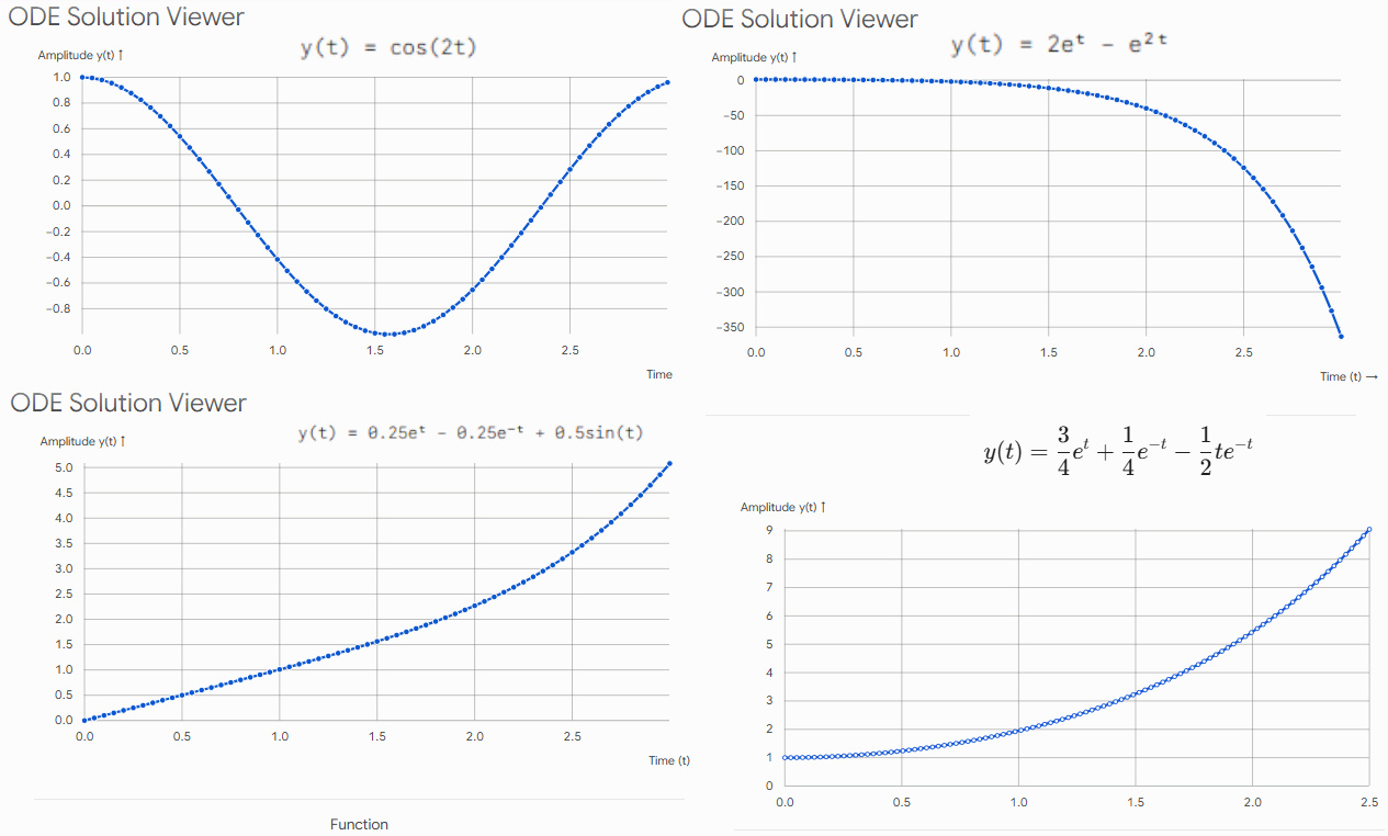
$y(t) = -\frac{1}{2}t e^{-t} + \frac{1}{4}e^{-t} + \frac{3}{4}e^{t}$. As $t \to +\infty$: $e^{t}$ dominates everything: $y(t) \sim \frac{3}{4}e^{t} \quad\Rightarrow\quad y(t) \to +\infty.$

Bibliography

1. NPTEL-NOC IITM, Introduction to Galois Theory.
2. Algebra, Second Edition, by Michael Artin.
3. LibreTexts, Calculus and Calculus 3e (Apex). Abstract and Geometric Algebra, Abstract Algebra: Theory and Applications (Judson).
4. Field and Galois Theory, by Patrick Morandi. Springer.
5. Michael Penn, and MathMajor.
6. Contemporary Abstract Algebra, Joseph, A. Gallian.
7. YouTube’s Andrew Misseldine: Calculus. College Algebra and Abstract Algebra.
8. MIT OpenCourseWare [18.03 Differential Equations, Spring 2006], YouTube by MIT OpenCourseWare.
9. Calculus Early Transcendentals: Differential & Multi-Variable Calculus for Social Sciences.