Now I am become Death, the destroyer of worlds, Robert Oppenheimer

Fourier Series

Linear First-Order Systems: The Matrix Approach

A general linear first-order system of two variables has the form:

$\begin{cases} x' = a(t)x + b(t)y + r_1(t) \\\\ y' = c(t)x + d(t)y + r_2(t) \end{cases}$ where:

$a(t), b(t), c(t)$, and $d(t)$ are functions of time $t$ (or constants in simpler cases).
$r_1(t)$ and $r_2(t)$ represent external forcing functions or inputs.
$x(t_0) = x_0$ and $y(t_0) = y_0$ are the initial conditions.

Fourier Series

Sketching Solutions of a Homogeneous Linear System with Complex Eigenvalues

Analyzing differential equations through phase portraits is a beautiful way to understand dynamic systems. Our goal is to solve the system, find the general solution, and sketch the trajectories to understand its behavior over time.

Example 1: A Counterclockwise Spiral Sink

Consider the following system of differential equations: $\begin{cases} x' = -x -y \\\ y' = 2x -3y \end{cases}$

Our goal is to solve this system, find the general solution, and sketch the trajectories of the solutions to understand the system’s behavior over time.

Step 1: Representing the System in Matrix Form. We can represent the system in the matrix form $\mathbf{x}' = A\mathbf{x}$, where: $\mathbf{x} = \begin{pmatrix} x \\ y \end{pmatrix}, \quad \mathbf{x}' = \begin{pmatrix} x' \\ y' \end{pmatrix}, \quad A = \begin{pmatrix} -1 & -1 \\ 2 & -3 \end{pmatrix}$

Step 2: Finding the Eigenvalues of Matrix A

To solve this system, we need to find the eigenvalues $\lambda$ and eigenvectors $\mathbf{v}$ of matrix $A$. The eigenvalues are found by solving the characteristic equation $\det(A - \lambda I) = 0$, where $I$ is the identity matrix.

$\det(A - \lambda I) = \begin{vmatrix} -1-\lambda & -1 \\ 2 & -3-\lambda \end{vmatrix} = (-1-\lambda)(-3-\lambda) - (-1)(2)$

Expanding this polynomial: $(\lambda+1)(\lambda+3) + 2 = \lambda^2 + 4\lambda + 3 + 2 = \lambda^2 + 4\lambda + 5 = 0$

Solving the characteristic equation using the quadratic formula: $\lambda = \frac{-4 \pm \sqrt{16 - 20}}{2} = \frac{-4 \pm \sqrt{-4}}{2} = -2 \pm i$

Step 3: Finding the Eigenvectors

We need to solve the equation $(A - \lambda I)\mathbf{v} = 0$.

Let’s use the first eigenvalue, $\lambda_1 = -2 + i$.

Substitute $\lambda_1$ into $A - \lambda I$, and we get: $\begin{pmatrix} -1 - (-2+i) & -1 \\ 2 & -3 - (-2+i) \end{pmatrix} = \begin{pmatrix} 1-i & -1 \\ 2 & -1-i \end{pmatrix}$

We now solve for the eigenvector $\mathbf{v}_1 = \begin{pmatrix} a_1 \\ a_2 \end{pmatrix}$: $\begin{pmatrix} 1-i & -1 \\ 2 & -1-i \end{pmatrix} \begin{pmatrix} a_1 \\ a_2 \end{pmatrix} = \begin{pmatrix} 0 \\ 0 \end{pmatrix}$

This gives us the system of equations:

$(1-i)a_1 - a_2 = 0 \implies a_2 = (1-i)a_1$
$2a_1 + (-1-i)a_2 = 0$

Both equations yield the same relationship. For the sake of convinience and simplicity, we can choose $a_1 = 1$, which gives $a_2 = 1 - i$. Thus, the eigenvector corresponding to $\lambda_1 = -2 + i$ is: $\mathbf{v}_1 = \begin{pmatrix} 1 \\ 1-i \end{pmatrix}$

Step 4: Constructing the General Solution

A complex solution to the system is given by $\mathbf{x} = e^{\lambda t}\mathbf{v}$.

Substituting our values: $\mathbf{x} = e^{(-2+i)t} \begin{pmatrix} 1 \\ 1-i \end{pmatrix}$

Using exponent rules and Euler’s formula ($e^{it} = \cos(t) + i\sin(t)$), we can expand this: $\mathbf{x} = e^{-2t} (\cos(t) + i\sin(t)) \left[ \begin{pmatrix} 1 \\ 1 \end{pmatrix} + i\begin{pmatrix} 0 \\ -1 \end{pmatrix} \right]$

Simplifying, and grouping the real and imaginary components, we get:

Real Part: $\mathbf{x}_{\text{real}} = e^{-2t} \left( \begin{pmatrix} 1 \\ 1 \end{pmatrix}\cos(t) - \begin{pmatrix} 0 \\ -1 \end{pmatrix}\sin(t) \right)$
Imaginary Part: $\mathbf{x}_{\text{imag}} = e^{-2t} \left( \begin{pmatrix} 1 \\ 1 \end{pmatrix}\sin(t) + \begin{pmatrix} 0 \\ -1 \end{pmatrix}\cos(t) \right)$

The general solution is a real-valued function, so we consider the real and imaginary parts separately. The real part provides one solution, and the imaginary part provides another. Therefore, the general solution is: $\boxed{\mathbf{x}(t) = c_1 e^{-2t} \begin{pmatrix} \cos(t) \\ \cos(t) + \sin(t) \end{pmatrix} + c_2 e^{-2t} \begin{pmatrix} \sin(t) \\ \sin(t) - \cos(t) \end{pmatrix}}$

Step 5: Sketching the Trajectories (Phase Portrait)

What does this solution look like geometrically?

The Shape (Oscillation): The sine and cosine terms tell us the curves are periodic and bounded ($e^{-2t}$ is a decaying exponential, too), forming ellipses or circles.
The Stability (Decay): The exponential term $e^{-2t}$ acts as a damping factor. Because $-2 < 0$, the amplitude of the trajectories decreases over time.
The Result: The system describes a spiral sink. As time progresses ($t \to \infty$), the trajectories spiral inward toward the origin $(0,0)$ (Figure v).

How do we know the direction of the spiral?

To find out if it rotates clockwise or counterclockwise, we calculate the system’s velocity vector at a simple test point, like $(1, 0)$.

$x' = - (1) - 0 = -1$ (motion to the left)
$y' = 2(1) - 3(0) = 2$ (motion upwards)

Since the velocity vector at $(1,0)$ is $\begin{pmatrix} -1 \\ 2 \end{pmatrix}$, the flow points up and to the left. This indicates a counterclockwise rotation around the origin.

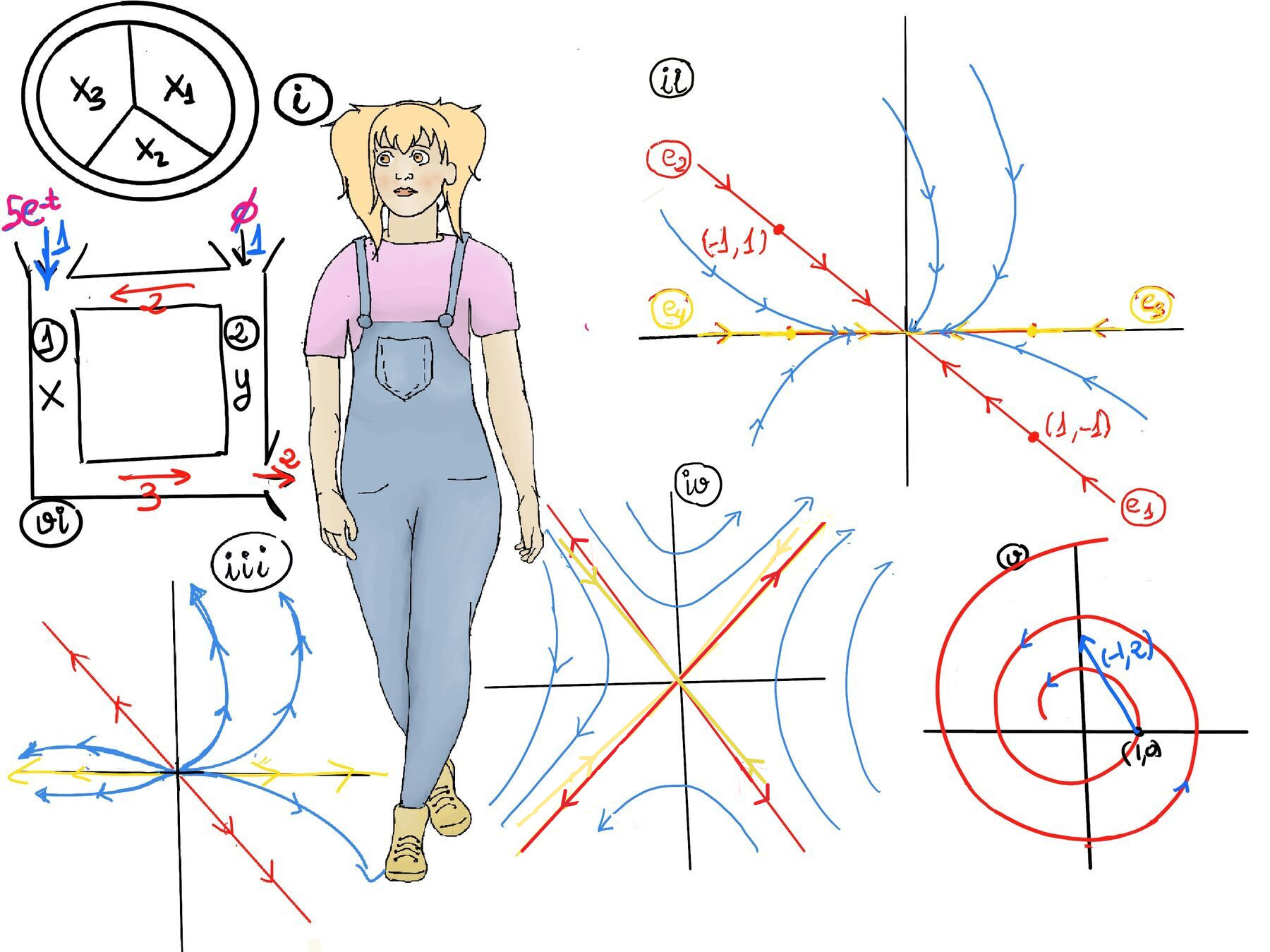
Sketching Solutions of 2x2 Homogeneous Linear System

Example 2: A Clockwise Spiral Sink

Let’s look at another homogeneous linear system defined by matrix $A$: $A = \begin{pmatrix} -2 & 3 \\ -3 & -2 \end{pmatrix}$

Step 1: Finding the Eigenvalues

We find the eigenvalue $\lambda$ by solving the characteristic equation: $\det \begin{pmatrix} -2-\lambda & 3 \\ -3 & -2-\lambda \end{pmatrix} = 0$

Expanding and simplifying: $(-2-\lambda)(-2-\lambda) - (3)(-3) = 0$

$(\lambda+2)^2 + 9 = 0 \implies (\lambda+2)^2 = -9 \implies \lambda+2 = \pm 3i$

Thus, the eigenvalues are $\lambda = -2 \pm 3i$.

Step 2: Analyzing the Behavior

Real Part ($\text{Re}(\lambda) = -2$): Since the real part is negative, the trajectories will decay over time, moving toward the origin.
Imaginary Part ($\text{Im}(\lambda) = \pm 3i$): The presence of the imaginary part indicates bounded, oscillatory behavior (spiraling).

Together, these dictate that the system exhibits a stable spiral sink.

The presence of the imaginary part ±3i indicates that the trajectories will be spirals (oscillatory bounded behaviour), causing the trajectories to spiral rather than move directly inward.

Step 3: Determining the Direction We compute the action of the matrix on the standard basis vector $\begin{pmatrix} 1 \\ 0 \end{pmatrix}$:

$$\begin{pmatrix} -2 & 3 \\ -3 & -2 \end{pmatrix} \begin{pmatrix} 1 \\ 0 \end{pmatrix} = \begin{pmatrix} -2 \\ -3 \end{pmatrix}$$

At the point $(1, 0)$, the vector points downwards and to the left. If you follow this arrow from the positive x-axis, it pulls you in a clockwise direction.

This homogeneous linear system is stable because the trajectories spiral inward towards the origin. The negative real part of the eigenvalues causes the trajectories to move towards the origin, and the presence of the imaginary part indicates that the trajectories are spirals. The system exhibits a stable spiral inward toward the origin in a clockwise direction (Refer to Figure i for a visual representation and aid in understanding it).

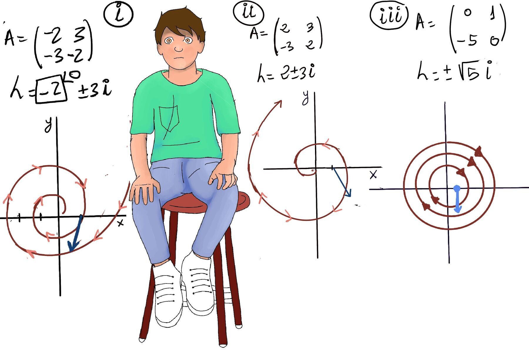
Sketch the following homogeneous linear system

Continuing our analysis of phase portraits, we now examine two different types of behaviors that emerge from complex eigenvalues: exponential growth (unstable spirals) and purely oscillatory motion (centers).

Example 3: A Clockwise Spiral Source

Consider the following system of differential equations represented by matrix $A$: $A = \begin{pmatrix} 2 & 3 \\ -3 & 2 \end{pmatrix}$

Step 1: Finding the Eigenvalues

We compute the characteristic equation $\det(A - \lambda I) = 0$: $\det \begin{pmatrix} 2-\lambda & 3 \\ -3 & 2-\lambda \end{pmatrix} = 0$

Expanding the determinant: $(2-\lambda)^2 - (-3)(3) = 0$

$(2-\lambda)^2 + 9 = 0 \implies (2-\lambda)^2 = -9 \implies 2-\lambda = \pm 3i$

Thus, the eigenvalues are: $\lambda = 2 \pm 3i$

Step 2: Analyzing the Behavior

Real Part ($\text{Re}(\lambda) = 2$): Because the real part is strictly positive ($2 > 0$), the system will experience exponential growth. The trajectories will move outward, away from the origin.
Imaginary Part ($\text{Im}(\lambda) = \pm 3i$): The presence of an imaginary part dictates oscillatory, bounded behavior. Combined with the exponential growth, the trajectories are forced into expanding spirals.

Conclusion: The system exhibits an unstable spiral source, meaning trajectories spiral outward, away from the origin as time progresses (moving away from the origin due to exponential growth).

Step 3: Determining the Direction

To determine the direction of the spiral, we compute the action of the matrix on the standard basis vector $\begin{pmatrix} 1 \\ 0 \end{pmatrix}$ (a point on the positive x-axis):

$$\begin{pmatrix} 2 & 3 \\ -3 & 2 \end{pmatrix} \begin{pmatrix} 1 \\ 0 \end{pmatrix} = \begin{pmatrix} 2 \\ -3 \end{pmatrix}$$

At the point $(1, 0)$, the velocity vector points to the right and downwards. Following this arrow from the positive x-axis indicates a clockwise rotation.

This homogeneous linear system is unstable because the trajectories spiral outwards away from the origin. The positive real part of the eigenvalues causes the trajectories to move away from the origin, and the presence of the imaginary part indicates that the trajectories are spirals. The system exhibits an unstable spiral (trajectories spiral outward from the origin) in a clockwise direction (Refer to Figure ii for a visual representation and aid in understanding it).