Sketching Solutions of Homogeneous Linear System 2

Behind this mask there is more than just flesh. Beneath this mask there is an idea… and ideas are bulletproof, Alan Moore

Linear First-Order Systems: The Matrix Approach

A general linear first-order system of two variables has the form:

$\begin{cases} x' = a(t)x + b(t)y + r_1(t) \\\\ y' = c(t)x + d(t)y + r_2(t) \end{cases}$ where:

• $a(t), b(t), c(t)$, and $d(t)$ are functions of time $t$ (or constants in simpler cases).
• $r_1(t)$ and $r_2(t)$ represent external forcing functions or inputs.
• $x(t_0) = x_0$ and $y(t_0) = y_0$ are the initial conditions.

Homogeneous Linear Systems with Constant Coefficients

Let’s explore homogeneous linear systems of first-order ordinary differential equations (ODEs) with constant coefficients. Specifically, we will return to our egg-cooling temperature model:

$\begin{cases} x' = -2x + 2y \\\\ y' = 2x - 5y \end{cases}$ where:

• we have swapped $T_1$ and $T_2$ for standard variables $x$ and $y$ for simplicity.
• x(t) and y(t) are the dependent variables (the state of the system).
• t is the independent variable (typically representing time).
• x’ = $\frac{dx}{dt}$ and y’ = $\frac{dy}{dt}$ denote the first derivatives of x(t) and y(t) respectively with respect to t.

This system of ODEs is classified as a homogeneous linear system because:

• The equations are perfectly linear with respect to $x$ and $y$ (no $x^2$, $xy$, or $\sin(x)$ terms).
• There are no standalone forcing terms, i.e., there are no constant terms or terms that depend exclusively on $t$ without being attached to $x$ or $y$.

In a previous article, we solved this exact system using the substitution method (converting it into a single second-order ODE). Our solution was: $\begin{cases} x = C_1e^{-t} + C_2e^{-6t} \\\ y = \frac{1}{2}C_1e^{-t} - 2C_2e^{-6t} \end{cases}$

While substitution works fine for 2x2 systems, it becomes messy, a computational nightmare for larger systems. Instead, we will solve this using the Eigenvalue and Eigenvector method. This powerful approach transforms the differential equations into an algebraic matrix problem, $\vec{x}' = A\vec{x}$, allowing us to find the general solution by simply identifying the matrix $A$’s eigenvalues ($\lambda$) and corresponding eigenvectors ($\vec{v}$).

Sketching a Stable Node (Sink)

Let’s analyze the following homogeneous linear system defined by matrix $A$: A = $(\begin{smallmatrix}-3 & 0\\\ 3 & -2\end{smallmatrix})$.

Using the eigenvalue method, the general solution is: $\vec{x} = C_1(\begin{smallmatrix}1\\\ -3\end{smallmatrix})e^{-3t} + C_2(\begin{smallmatrix} 0\\\ 1\end{smallmatrix})e^{-2t}$

• For $\lambda_1 = -3 < 0$: The corresponding eigenvector is $\begin{pmatrix} 1 \\ -3 \end{pmatrix}$. This means the pure trajectory associated with this eigenvalue lies precisely along the straight line $y = -3x$.

• For $\lambda_2 = -2 < 0$: The corresponding eigenvector is $\begin{pmatrix} 0 \\ 1 \end{pmatrix}$. The pure trajectory associated with this eigenvalue lies precisely along the line $x = 0$ (the y-axis).

Since both eigenvalues are negative, all trajectories in the vicinity of the origin will converge towards it as time progresses ($t \to \infty$), making the origin a stable node or sink.

To sketch the curved trajectories for points not starting exactly on those lines, we compare the decay rates. As $t \to \infty$, the term associated with the “slow” eigenvalue ($\lambda_2 = -2$) decays slower than the term associated with the “fast” eigenvalue ($\lambda_1 = -3$). Therefore, the $e^{-2t}$ term will eventually dominate the system’s behavior as it approaches the origin.

Sketching rule

1. Along the lines $y = -3x$ and the y-axis, trajectories move perfectly straight toward the origin.
2. For any other initial point, the trajectory is initially influenced by both eigenvectors. However, as t increases, the slower decaying $e^{-2t}$ term dominates, causing the trajectory to converge to the origin tangent to the direction of the eigenvector $\begin{pmatrix} 0 \\ 1 \end{pmatrix}$ (the y-axis).
3. Since all trajectories move towards the origin, the system is strictly stable. Refer to Figure B for a visual representation.

Sketching a Saddle Point

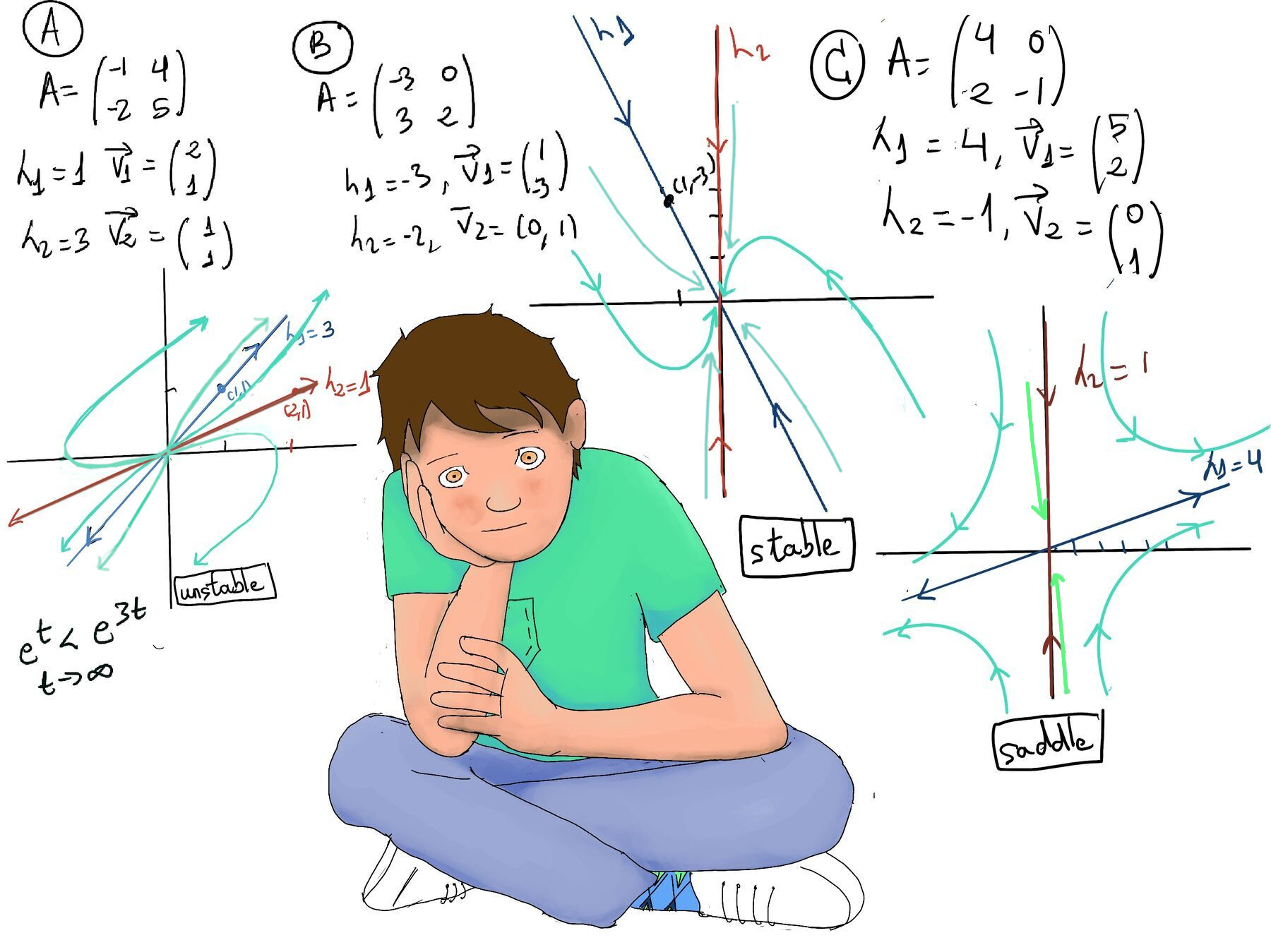
Now let’s sketch a system with mixed signs in its eigenvalues: A = $(\begin{smallmatrix}4 & 0\\\ 2 & -1\end{smallmatrix})$.

The general solution is: $\vec{x} = C_1(\begin{smallmatrix}5\\\ 2\end{smallmatrix})e^{4t} + C_2(\begin{smallmatrix} 0\\\ 1\end{smallmatrix})e^{-t}$

• For $\lambda_1 = 4 > 0$: The eigenvector is $\begin{pmatrix} 5 \\ 2 \end{pmatrix}$. Trajectories on the line $y = \frac{2}{5}x$ will move away from the origin.

  Every eigenvector defines a straight line through the origin along which the flow moves. If $A v_1 = 4 v_1$, then the direction of $v_1$ is invariant under the flow. So any solution of the form $x(t) = C_1 v_1 e^{4t}$ stays on the line spanned by $v_1$. The line spanned by $v_1 = \begin{pmatrix}5 \ 2\end{pmatrix}, [C_2 = 0]$ is all multiples of: $v_1, \begin{pmatrix}5s \ 2s\end{pmatrix},\quad s\in\mathbb{R}$. From $x = 5s,\qquad y = 2s,$ we eliminate (s): $s = \frac{x}{5} \quad\Rightarrow\quad y = 2\left(\frac{x}{5}\right) = \frac{2}{5}x$.

• For $\lambda_2 = -1 < 0$: The eigenvector is $\begin{pmatrix} 0 \\ 1 \end{pmatrix}$. Trajectories on the line $x = 0$ (the y-axis) will move towards the origin.

The term $C_1 \begin{pmatrix} 5 \\ 2 \end{pmatrix} e^{4t}$ grows exponentially, while $C_2 \begin{pmatrix} 0 \\ 1 \end{pmatrix} e^{-t}$ decays exponentially. Because one eigenvalue pulls trajectories in and the other pushes them out, the origin acts as a saddle point in the phase portrait.

Sketching rule

1. Any initial point lying exactly on the y-axis will move towards the origin as $t \to \infty$, due to the decaying term $e^{-t}$.
2. Any initial point lying exactly on $y = \frac{2}{5}x$ will move away from the origin as $t \to \infty$, since the term $e^{4t}$ grows exponentially.
3. For all other trajectories (points not perfectly on the y-axis), they will initially be influenced by both eigenvectors, but eventually, the growing $e^{4t}$ term will dominate, causing the trajectory to turn and align with the direction of $\begin{pmatrix} 5 \\ 2 \end{pmatrix}$ and diverge form the origin. They sweep in and then sweep out, creating a characteristic hyperbola-like shape.

Refer to Figure C for a visual representation of this saddle behavior.

Sketching an Unstable Node (Source)

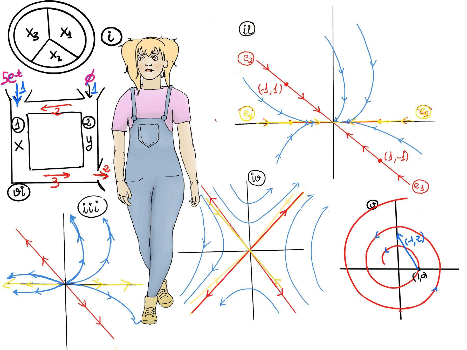
Finally, let’s analyze a system where both eigenvalues are positive. Suppose our general solution is: $\vec{x} = C_1(\begin{smallmatrix}1\\\ -1\end{smallmatrix})e^{3t} + C_2(\begin{smallmatrix} 1\\\ 0\end{smallmatrix})e^{t}$

This situation is the mirror opposite of the stable sink we discussed earlier. Because both eigenvalues are positive ($\lambda_1 = 3$ and $\lambda_2 = 1$), the system features an unstable node (or source) at the origin, where all trajectories diverge away from it over time.

To sketch the curves, we again look at dominance, but this time for exponential growth:

• Behavior as $t \to \infty$: The dominant term is $C_1 \begin{pmatrix} 1 \\ -1 \end{pmatrix} e^{3t}$ because it grows much faster than $e^t$. This implies that as time progresses forward, all trajectories (except those starting exactly on the x-axis) will move away from the origin eventually become parallel to the line $y = -x$.
• Behavior as $t \to -\infty$ (Near the origin): If we trace the trajectories backward to see how they emerge from the origin, the “slow” term $C_2 \begin{pmatrix} 1 \\ 0 \end{pmatrix} e^{t}$ dictates the shape. Trajectories emerge from the origin tangent to the eigenvector $\begin{pmatrix} 1 \\ 0 \end{pmatrix}$ (the x-axis).

Refer to Figure iii for a visual representation of how these trajectories emerge horizontally from the origin and then bend sharply to follow the line $y = -x$.

Step-by-Step Example: An Advertising War (Saddle Point)

Let’s put everything together to fully solve and sketch a new homogeneous linear system with constant coefficients. Consider the following system of differential equations: $\begin{cases} x' = -x +3y \\\ y' = 5x -3y \end{cases}$

Step 1: Representing the System in Matrix Form

Our goal is to solve this system, find the general solution, and sketch the trajectories of the solutions to understand the system’s behavior over time.

We can express the system in matrix form as $\vec{x}' = A\vec{x}$ where A = $(\begin{smallmatrix}-1 & 3\\\ 5 & -3\end{smallmatrix})$ and $\vec{x} = (\begin{smallmatrix}x\\\ y\end{smallmatrix})$ This matrix equation perfectly encapsulates the system of differential equations.

To solve this system, we must find the eigenvalues and eigenvectors of the matrix A.

Step 2: Finding the Eigenvalues of Matrix A

The characteristic equation is derived from the determinant of $A - \lambda I = 0$, where I is the identity matrix and $\lambda$ represents the eigenvalues.

To find the eigenvalues, we solve the characteristic equation: $|A - \lambda I| = \vert\begin{smallmatrix}-1-λ & 3\\\ 5 & -3-λ\end{smallmatrix}\vert$

Expanding the determinant: $|A - \lambda I| = 0 \iff \lambda^2 + 4\lambda - 12 = 0$.

Factoring the quadratic equation yields: $(\lambda + 6)(\lambda - 2) = 0$. Thus, our two eigenvalues are $\lambda_1 = -6$ and $\lambda_2 = 2$. Because they have opposite signs, we immediately know this will be a saddle point.

Step 3: Finding the Eigenvectors

We will find an eigenvector corresponding to each eigenvalue $\lambda$ by solving $(A - \lambda I)\vec{v} = 0$.

• For Eigenvalue $\lambda_1 = -6$:

$\begin{pmatrix} -1 - (-6) & 3 \\ 5 & -3 - (-6) \end{pmatrix} \begin{pmatrix} v_1 \\ v_2 \end{pmatrix} = \begin{pmatrix} 5 & 3 \\ 5 & 3 \end{pmatrix} \begin{pmatrix} v_1 \\ v_2 \end{pmatrix} = \begin{pmatrix} 0 \\ 0 \end{pmatrix}$

This yields the redundant system $5v_1 + 3v_2 = 0$. This indicates infinite solutions along a line where $v_1 = -\frac{3}{5}v_2$. To avoid using fractions, we can choose $v_2 = -5$ for simplicity, which gives $v_1 = 3$.

The stable eigenvector is $\vec{v}_1 = \begin{pmatrix} 3 \\ -5 \end{pmatrix}$.

• For Eigenvalue $\lambda_2 = 2$:

$$\begin{pmatrix} -1 - 2 & 3 \\ 5 & -3 - 2 \end{pmatrix} \begin{pmatrix} v_1 \\ v_2 \end{pmatrix} = \begin{pmatrix} -3 & 3 \\ 5 & -5 \end{pmatrix} \begin{pmatrix} v_1 \\ v_2 \end{pmatrix} = \begin{pmatrix} 0 \\ 0 \end{pmatrix}$$

This yields the system $-3v_1 + 3v_2 = 0$, which simplifies to $v_1 = v_2$. We can choose $v_1 = 1$ and $v_2 = 1$.

The unstable eigenvector is $\vec{v}_2 = \begin{pmatrix} 1 \\ 1 \end{pmatrix}$.

Step 4: Constructing the General Solution

The general solution to the system is a linear combination of the eigenvectors multiplied by the exponential functions of their corresponding eigenvalues: $\vec{x}(t) = C_1 \vec{v}_1 e^{\lambda_1 t} + C_2 \vec{v}_2 e^{\lambda_2 t}$

Substituting our findings yields $\begin{pmatrix} x(t) \ y(t) \end{pmatrix} = C_1 \begin{pmatrix} 3 \ -5 \end{pmatrix} e^{-6t} + C_2 \begin{pmatrix} 1 \ 1 \end{pmatrix} e^{2t}

This gives us the parametric equations: $x(t) = 3C_1e^{-6t} + C_2e^{2t}$ and $y(t) = -5C_1e^{-6t} + C_2e^{2t}$

Step 5: Analyzing the Behavior of the Solutions

1. The Saddle Point: Because the eigenvalues have opposite signs ($-6$ and $2$), the origin is a saddle point (Refer to Figure iv for a visual representation and aid in understanding it).
2. Unstable Direction ($t \to \infty$): For large positive $t$, the term $C_2 \begin{pmatrix} 1 \\ 1 \end{pmatrix} e^{2t}$ dominates the system because of the positive eigenvalue $\lambda_2 = 2$. Trajectories are pushed away from the origin along the line spanned by the unstable eigenvector $\begin{pmatrix} 1 \\ 1 \end{pmatrix}$. This corresponds to moving outwards along the line $y = x$.
3. Stable Direction ($t \to -\infty$): For large negative $t$, or when observing the system in reverse, the term $C_1 \begin{pmatrix} 3 \\ -5 \end{pmatrix} e^{-6t}$ dominates. The trajectories approach the origin strictly along the direction of the stable eigenvector $\begin{pmatrix} 3 \\ -5 \end{pmatrix}$, which corresponds to the line $y = -\frac{5}{3}x$ (trajectories are attracted to the origin along this direction in backward time).
4. General Trajectories: The trajectories between these two distinct straight-line directions exhibit curved, hyperbola-like behavior. They sweep inward toward the origin along the stable manifold ($y = -\frac{5}{3}x$) and then diverge sharply outward along the unstable manifold ($y = x$) as $t \to \infty$.

Real-World Application: This mathematical model can represent a scenario where two competing companies are engaged in an advertising war. The saddle point nature implies that finding a balanced, sustainable strategy (staying at the origin) is incredibly precarious. The mathematics suggest that slight perturbations will cause the system to snap into an unstable direction—meaning both companies are driven either toward aggressive, runaway overspending (growth along $y=x$) or rapid simultaneous decline.

Bibliography

1. NPTEL-NOC IITM, Introduction to Galois Theory.
2. Algebra, Second Edition, by Michael Artin.
3. LibreTexts, Calculus and Calculus 3e (Apex). Abstract and Geometric Algebra, Abstract Algebra: Theory and Applications (Judson).
4. Field and Galois Theory, by Patrick Morandi. Springer.
5. Michael Penn, and MathMajor.
6. Contemporary Abstract Algebra, Joseph, A. Gallian.
7. YouTube’s Andrew Misseldine: Calculus. College Algebra and Abstract Algebra.
8. MIT OpenCourseWare [18.03 Differential Equations, Spring 2006], YouTube by MIT OpenCourseWare.
9. Calculus Early Transcendentals: Differential & Multi-Variable Calculus for Social Sciences.