Sketching Solutions of 2x2 Homogeneous Linear Systems

The first principle is that you must not fool yourself – and you are the easiest person to fool, Richard Feynman

Linear First-Order Systems: The Matrix Approach

A general linear first-order system of two variables has the form:

$\begin{cases} x' = a(t)x + b(t)y + r_1(t) \\\\ y' = c(t)x + d(t)y + r_2(t) \end{cases}$ where:

• $a(t), b(t), c(t)$, and $d(t)$ are functions of time $t$ (or constants in simpler cases).
• $r_1(t)$ and $r_2(t)$ represent external forcing functions or inputs.
• $x(t_0) = x_0$ and $y(t_0) = y_0$ are the initial conditions.

Homogeneous Linear Systems with Constant Coefficients

Let’s explore homogeneous linear systems of first-order ordinary differential equations (ODEs) with constant coefficients. Specifically, we will return to our egg-cooling temperature model:

$\begin{cases} x' = -2x + 2y \\\\ y' = 2x - 5y \end{cases}$ where:

• We have swapped $T_1$ and $T_2$ for standard variables $x$ and $y$ for simplicity.
• x(t) and y(t) are the dependent variables.
• t is the independent variable (typically representing time).
• x’ = $\frac{dx}{dt}$ and y’ = $\frac{dy}{dt}$ denote the first derivatives of x(t) and y(t) with respect to t.

The given system of ODE’s is a homogeneous linear system because:

• The equations are perfectly linear with respect to $x$ and $y$.
• There are no standalone forcing terms depending only on $t$.

There are no constant or forcing terms (i.e., terms that do not depend on x or y).

In a previous section, we solved this exact system using the substitution method (converting it into a single second-order ODE). Our solution was: $\begin{cases} x = C_1e^{-t} + C_2e^{-6t} \\\ y = \frac{1}{2}C_1e^{-t} - 2C_2e^{-6t} \end{cases}$

While substitution works for 2x2 systems, it becomes computationally messy (nightmarish) for larger systems. Instead, we will solve this using the Eigenvalue and Eigenvector method. This approach transforms the system into an algebraic problem, allowing us to find the general solution by identifying the system’s eigenvalues and corresponding eigenvectors.

Sketching Solutions of a 2x2 Homogeneous Linear System with Constant Coefficients

Let’s analyze and sketch the phase portraits of several homogeneous linear systems. Each system is defined by a matrix A and its corresponding general solution.

The Tourism Competition Model

This model considers the competition between Massachusetts and New Hampshire regarding their tourism advertising budgets. We model how deviations from their average (baseline) advertising budgets evolve over time. Let:

• x(t): Departure of Massachusetts’ tourism budget from its normal (average) level at time t.
• y(t): Departure of New Hampshire’s tourism budget from its normal (average) level at time t.

The underlying idea is that if a state spends more than usual on tourism in a given year, there’s internal political pressure to spend less in the future to balance other needs (e.g., education, military, infrastructure, or social services; represented by -x, -3y respectively). Conversely, if a state spends less than average, there’s pressure from local businesses and entrepreneurs to increase tourism advertising.

Because the states are also competing for the same tourists, we must also introduce interaction terms. We model the situation with the following system of differential equations:

We model the situation with the following system:

$\begin{cases} x' = -x +by \\\ y' = cx -3y \end{cases}$

The given system of differential equations represents a model for competition, potentially between two entities such as nations in a conflict or companies in a market. Here, x and y represent the states of the two competing entities, and b and c are positive constants that describe the competitive interaction between them.

For our specific case study, we will analyze the following dynamic:

$\begin{cases} x' = -x + 2y \\\ y' = -3y \end{cases}$

• Massachusetts ($x'$): The rate of change in its budget depends negatively on its own current deviation ($-x$) and positively on New Hampshire’s current deviation ($+2y$). If Massachusetts is over budget, there’s pressure to decrease spending ($-x$). However, if New Hampshire is heavily advertising ($+2y$), Massachusetts feels competitive pressure to increase its own budget ($+2y$).
• New Hampshire ($y'$): Its rate of change depends entirely on its own current deviation ($-3y$) and is independent of Massachusetts’ budget (x). The absence of an $x$ term implies that New Hampshire does not react to Massachusetts' actions.

This dynamic can be rewritten in matrix form as $x' = Ax$ where $\vec{x} = \begin{pmatrix} x \\ y \end{pmatrix}$ and the coefficient matrix is: A = $(\begin{smallmatrix}-1 & 2\\\ 0 & -3\end{smallmatrix})$

Finding Eigenvalues and Eigenvectors

To solve this system, we must find the eigenvalues ($\lambda$) and eigenvectors ($\vec{v}$) of the matrix $A$.

The characteristic equation is derived from the determinant of $A - \lambda I$, where I is the identity matrix and $\lambda$ represents the eigenvalues.

To find the eigenvalues, we solve the characteristic equation: $\det(A - \lambda I) = 0$: $\begin{vmatrix} -1 - \lambda & 2 \\ 0 & -3 - \lambda \end{vmatrix} = (-1 - \lambda)(-3 - \lambda) - (2)(0) = 0$

Expanding this yields: $\lambda^2 + 4\lambda + 3 = 0$

Factoring the quadratic gives: $(\lambda + 3)(\lambda + 1) = 0$

Thus, our eigenvalues are $\lambda_1 = -3$ and $\lambda_2 = -1$. Next, we find the corresponding eigenvectors by solving $(A - \lambda I)\vec{v} = 0$.

• For Eigenvalue $\lambda_1 = -3$:

$\begin{pmatrix} -1 - (-3) & 2 \\ 0 & -3 - (-3) \end{pmatrix} \begin{pmatrix} v_1 \\ v_2 \end{pmatrix} = \begin{pmatrix} 2 & 2 \\ 0 & 0 \end{pmatrix} \begin{pmatrix} v_1 \\ v_2 \end{pmatrix} = \begin{pmatrix} 0 \\ 0 \end{pmatrix}$

This gives the equation $2v_1 + 2v_2 = 0$, meaning $v_1 = -v_2$. Choosing (wisely) $v_2 = -1$, it gives $v_1 = 1$.

The first eigenvector corresponding to $\lambda_1 = -3$ is $\vec{v}_1 = \begin{pmatrix} 1 \\ -1 \end{pmatrix}$.

• For Eigenvalue $\lambda_2 = -1$:

$$\begin{pmatrix} -1 - (-1) & 2 \\ 0 & -3 - (-1) \end{pmatrix} \begin{pmatrix} v_1 \\ v_2 \end{pmatrix} = \begin{pmatrix} 0 & 2 \\ 0 & -2 \end{pmatrix} \begin{pmatrix} v_1 \\ v_2 \end{pmatrix} = \begin{pmatrix} 0 \\ 0 \end{pmatrix}$$

This gives the equation $2v_2 = 0$, so $v_2 = 0$. The value of $v_1$ is a free variable; so we choose $v_1 = 1$ for simplicity.

Therefore, the second eigenvector corresponding to $\lambda_2 = -1$ is $\vec{v}_2 = \begin{pmatrix} 1 \\ 0 \end{pmatrix}$.

The General Solution and Phase Portrait

The general solution to the system is a linear combination of the solutions corresponding to each eigenvalue (the eigenvectors multiplied by their exponential decay terms): $(\begin{smallmatrix}x\\\ y\end{smallmatrix}) = C_1α_1e^{λ_1t} + C_2α_2e^{λ_2t} =[\text{Substituting the eigenvalues and eigenvectors}] C_1(\begin{smallmatrix}1\\\ -1\end{smallmatrix})e^{-3t} + C_2(\begin{smallmatrix} 1\\\ 0\end{smallmatrix})e^{-t}$

This corresponds or translates to the system: $\begin{cases} x(t) = c_1e^{-3t}+ c_2e^{-t} \\\ y(t) = -c_1e^{-3t} \end{cases}$

To sketch the solutions, we examine the behavior for different values of $C_1$ and $C_2$ ($C_1 = \pm 1, 0; C_2 = \pm 1, 0$), and then fill in the rest.

• $e_1$: $c_1 = 1, c_2 = 0$ (in reality $c_1 \gt 0, c_2 = 0$). In this case, $x = e^{-3t}, y = -e^{-3t}$. $t = 0 \implies (x, y) = (1, -1)$. As t increases, it is always in the direction of $(\begin{smallmatrix}1\\\ -1\end{smallmatrix})$, meaning the trajectory lies along the line y = -x (approaching the origin faster due to the exponential term), but decreasing in length by $e^{-3t}$. The eigenvector $(\begin{smallmatrix}1\\\ -1\end{smallmatrix})$ determines the direction on which it travels and the eigenvalue determine which way it goes. If the eigenvalue is negative ($\lambda = -3$), it is approaching the origin as t increases. Refer to Figure ii for a visual representation and aid in understanding it.

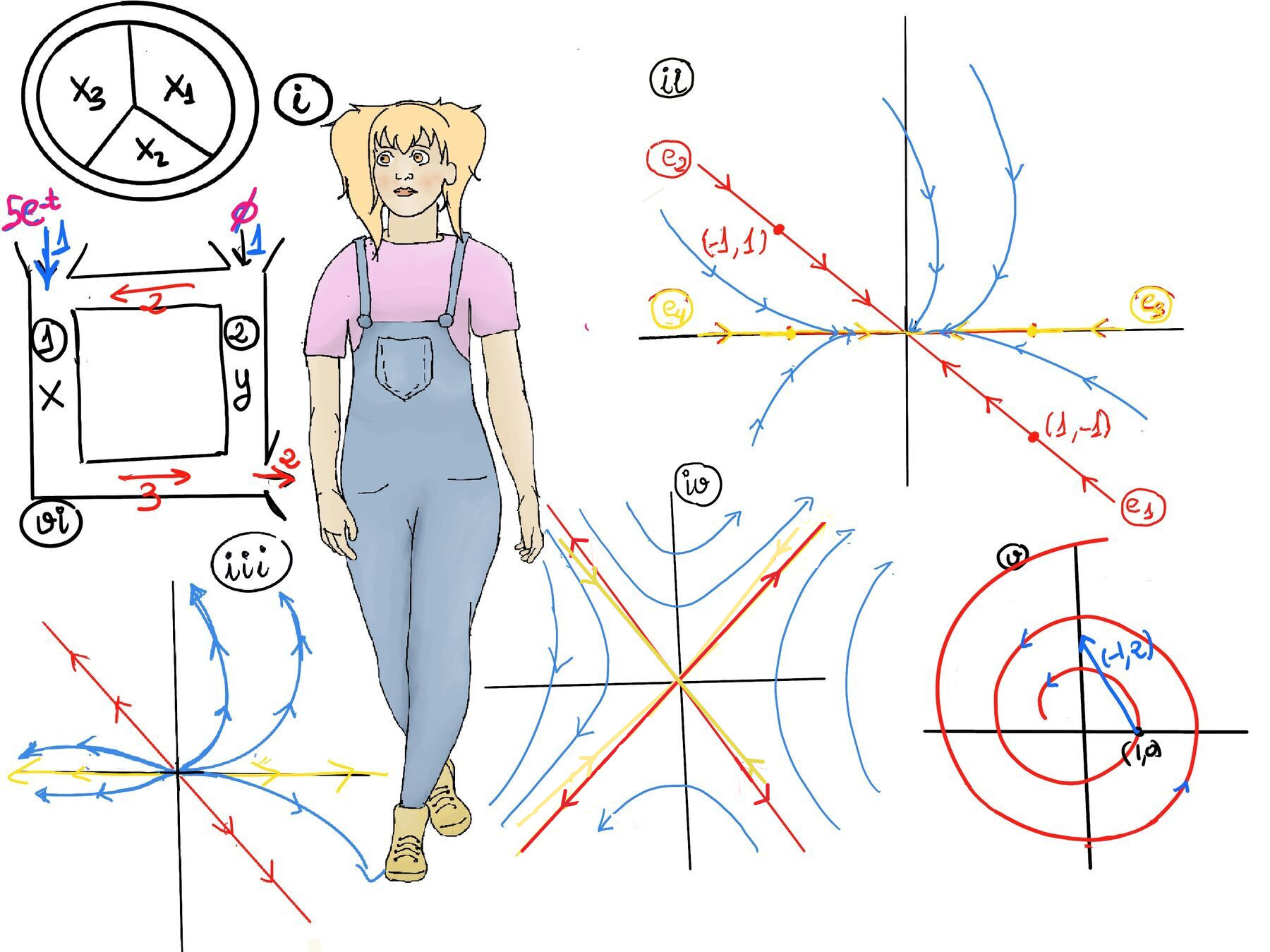
• $e_2: c_1 = -1, c_2 = 0$. Similarly, $x = -e^{-3t}, y = e^{-3t}$. $t = 0 \implies (x, y) = (-1, 1)$. As t increases, it is always in the direction of $(\begin{smallmatrix}-1\\\ 1\end{smallmatrix})$, meaning the trajectory lies along the line y = -x, but decreasing in length by $e^{-3t}$.

• $e_3: c_1 = 0, c_2 = 1$. $x = e^{-t}, y = 0$. $t = 0 \implies (x, y) = (1, 0)$. As t increases, t is always in the direction of $(\begin{smallmatrix}1\\\ 0\end{smallmatrix})$, so the trajectory lies along the x-axis, moving towards the origin as t increases.

• $e_4: c_1 = 0, c_2 = -1$. $x = -e^{-t}, y = 0$. $t = 0 \implies (x, y) = (-1, 0)$. As t increases, t is always in the direction of $(\begin{smallmatrix}-1\\\ 0\end{smallmatrix})$. The trajectory lies along the negative x-axis, also approaching the origin.

Long-Term Behavior and Stability Analysis

Because both eigenvalues are negative ($\lambda = -3$ and $\lambda = -1$), all trajectories —regardless of their starting initial conditions— converge toward the origin as $t \to \infty$, indicating that the origin is a sink node, a stable equilibrium point.

The mathematical analysis shows that the system is strictly stable and naturally converges to equilibrium. Both states’ advertising budgets will eventually revert to their normal, baseline averages.

Since the functions involved in the differential equations are continuous, the resulting velocity field is continuous. This implies that small changes in the state (values of x and y) lead to small changes in their rates of change, resulting in smooth trajectories. Consequently, the trajectories do not exhibit abrupt changes; instead, they evolve smoothly over time.

To understand the shape of these curves, we look at dominant terms. Suppose t = 10; $e^{-10}$ is indeed a very small number, but it is vastly larger than $e^{-30}$. As $t \to \infty$, the $e^{-3t}$ term decays much faster than $e^{-t}$. Therefore, after a long time, the behavior of the system is dominated by the 'slow' eigenvalue $\lambda_2 = -1$. As trajectories approach the origin, they flatten out and become tangent to the x-axis, because $y(t)$ reaches zero much faster than $x(t)$.

In real-world terms, New Hampshire ($y$) aggressively returns its budget to normal, while Massachusetts ($x$) lags behind, still trying to correct for its competitive reactions. However, despite different initial responses to changes in advertising budgets, both Massachusetts and New Hampshire eventually revert to their normal budgets over time, indicating that peace (or balance) in tourism advertising is eventually restored.

Classifying the Equilibrium: Nodes

A node is a specific type of equilibrium point (also called a fixed point) where all solution trajectories either strictly converge towards the point (approach the point) or strictly diverge away from it as as time progresses. Depending on the direction of the trajectories, nodes can be further classified as sinks or sources.

• A sink node (stable) is an equilibrium point where all nearby trajectories in the phase plane move towards the node (they are pulled inward) as time progresses ($t \to \infty$). When a node is located at the origin (0,0) and all trajectories in its vicinity converge towards this point over time, it is specifically referred to as a sink or sink node. This behavior indicates that the system is stable, as perturbations from the equilibrium point will decay over time, bringing the system back to equilibrium (any perturbation will naturally correct itself).

• A source node (unstable) is an equilibrium point where all nearby trajectories in the phase plane move away from the node as time progresses (i.e., as $t \to \infty$). This happens when eigenvalues are positive. This behavior signifies that the system is unstable, as small perturbations from the equilibrium point will grow over time, causing the system to diverge from equilibrium (small changes will cause the system to spiral out of control, diverging infinitely from equilibrium).

Sketching the Phase Portrait of a Homogeneous Linear System

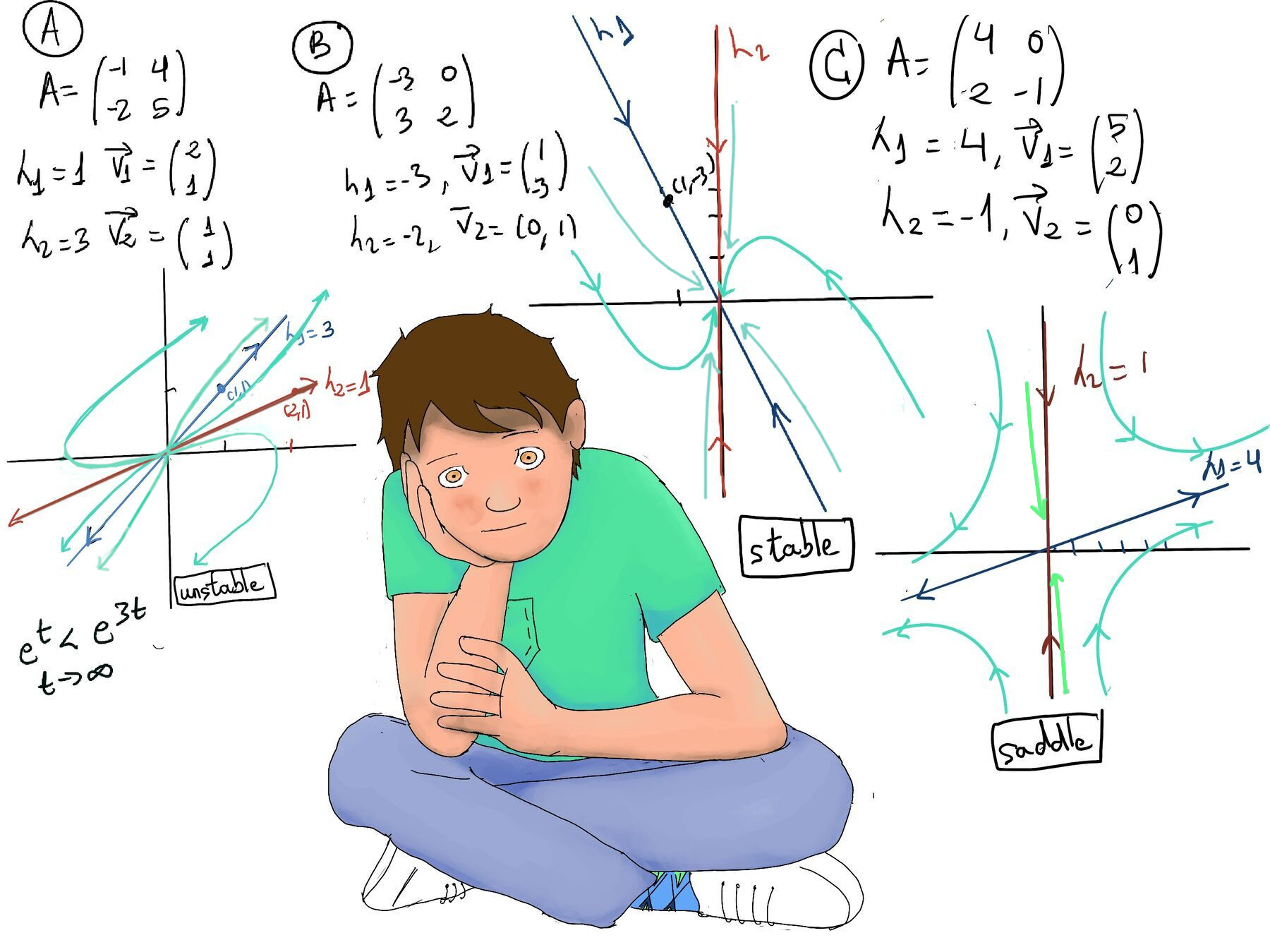
Let’s analyze the behavior of a linear system defined by the matrix: $A = \begin{pmatrix} -1 & 4 \\ -2 & 5 \end{pmatrix}$

The general solution to this system is given by the linear combination of its eigen-components: $\vec{x}(t) = C_1 \begin{pmatrix} 2 \\ 1 \end{pmatrix} e^t + C_2 \begin{pmatrix} 1 \\ 1 \end{pmatrix} e^{3t}$

To sketch the phase portrait accurately, we must examine the straight-line solutions (determined by the eigenvectors) and the general curved trajectories (determined by the interplay of the eigenvalues).

The Straight-Line Trajectories (Eigendirections)

• For $\lambda_1 = 1 > 0$: The corresponding eigenvector is $\begin{pmatrix} 2 \\ 1 \end{pmatrix}$. This means that the trajectory associated with this eigenvalue lies along the line y = $\frac{1}{2}x$ and also if the system starts on the line $y = \frac{1}{2}x$, it will stay on this line forever. Because $\lambda_1$ is positive, a particle on this line will move away from the origin as $t$ increases.

• For $\lambda_2 = 3 > 0$: The corresponding eigenvector is $\begin{pmatrix} 1 \\ 1 \end{pmatrix}$. This means that the trajectory associated with this eigenvalue lies along the line y = x and also if the system starts on the line $y = x$, it will also travel along this line, moving away from the origin as $t$ increases.

Stability Classification

Since both eigenvalues are positive ($\lambda_1 = 1, \lambda_2 = 3$), all trajectories in the vicinity of the origin will diverge away from it as time progresses, making the origin an unstable node or source. Any slight deviation from the equilibrium point at $(0,0)$ will grow exponentially.

Dominance and Trajectory Shape

To sketch the curves for points that do not start exactly on those two lines, we have to look at which term dominates the solution at different times:

• Behavior Far from the Origin ($t \to \infty$): As $t$ increases, both $e^t$ and $e^{3t}$ grow, but $e^{3t}$ grows significantly faster. Therefore, the term $C_2 \begin{pmatrix} 1 \\ 1 \end{pmatrix} e^{3t}$ will strongly dominate the behavior of the system. For any initial point not lying on the straight-line trajectories, it will initially be influenced by both eigenvectors. However, as t increases, the rapidly growing $e^{3t}$ term forces the trajectory to align almost perfectly parallel with the direction of the eigenvector$\begin{pmatrix} 1 \\ 1 \end{pmatrix}$. This results in rapid growth roughly along the line $y = x$.

• Behavior Near the Origin ($t \to -\infty$): If we trace the trajectories backward in time toward the origin, $e^{3t}$ decays to zero much faster than $e^t$. This means near the origin, the “slow” term $C_1 \begin{pmatrix} 2 \\ 1 \end{pmatrix} e^t$ dictates the shape. As trajectories emerge from the origin, they do so tangent to the line $y = \frac{1}{2}x$.

Conclusion:

Since all trajectories move away from the origin, the system is classified as strictly unstable. Trajectories emerge from the origin tangent to the slow eigenvector line ($y = \frac{1}{2}x$) and eventually bend to become parallel to the fast eigenvector line ($y = x$). Refer to Figure A for a visual representation.

Bibliography

1. NPTEL-NOC IITM, Introduction to Galois Theory.
2. Algebra, Second Edition, by Michael Artin.
3. LibreTexts, Calculus and Calculus 3e (Apex). Abstract and Geometric Algebra, Abstract Algebra: Theory and Applications (Judson).
4. Field and Galois Theory, by Patrick Morandi. Springer.
5. Michael Penn, and MathMajor.
6. Contemporary Abstract Algebra, Joseph, A. Gallian.
7. YouTube’s Andrew Misseldine: Calculus. College Algebra and Abstract Algebra.
8. MIT OpenCourseWare [18.03 Differential Equations, Spring 2006], YouTube by MIT OpenCourseWare.
9. Calculus Early Transcendentals: Differential & Multi-Variable Calculus for Social Sciences.