General Homogeneous Linear Systems. Wronskian, Fundamental Matrix, and Centers.

Quantity has its own quality, Joseph Stalin

General Homogeneous Linear System

In the study of differential equations —particularly in advanced calculus (Calculus III/IV) and linear algebra— homogeneous linear systems are fundamental. These systems allow us to model complex, multi-variable dynamical behaviors found in physics, engineering, ecology, and economics.

Specifically, we focus on first-order systems of the form: $\vec{x}' = A\vec{x}$ where:

• $\vec{x}(t)$ is a vector-valued function of unknown variables, typically $\vec{x}(t) = \begin{pmatrix} x(t) \\ y(t) \end{pmatrix}$.
• $A$ is a constant $2 \times 2$ coefficient matrix, $A = \begin{pmatrix} a_{11} & a_{12} \\ a_{21} & a_{22} \end{pmatrix}$.
• $\vec{x}'(t)$ denotes the derivative of $\vec{x}(t)$ with respect to time $t$.

To find the general solution to this system, we must understand the core concepts of the Principle of Superposition, linear independence, the Wronskian determinant, and the fundamental matrix.

The General Solution

Because differentiation is a linear operation, these systems obey the Principle of Superposition. This gives rise to the primary theorem for solving homogeneous systems.

Theorem (General Solution). The general solution to the system $\vec{x}' = A\vec{x}$ can be expressed as a linear combination of two linearly independent solutions: $\vec{x}(t) = c_1\vec{x}_1(t) + c_2\vec{x}_2(t)$ where $c_1$ and $c_2$ are arbitrary constants.

1. Fundamental Solutions: The vectors $\vec{x}_1(t)$ and $\vec{x}_2(t)$ are called a fundamental set of solutions because they form a basis for the entire solution space of the differential equation. Any possible solution can be constructed by mixing these two fundamental building blocks.
2. Linear Independence: Two solutions are linearly independent if one is not a constant scalar multiple of the other. Mathematically, there is no constant $k$ such that $\vec{x}_2(t) = k\vec{x}_1(t)$ for all $t$. This ensures our two solutions point in different “functional directions,” allowing them to span the full 2D solution space.
3. Constants $c_1$ and $c_2$: These are determined by the Initial Value Problem (IVP). If we are given an initial state, such as $\vec{x}(t_0) = \vec{x}_0$, we can solve for $c_1$ and $c_2$ algebraically to find the specific trajectory of the system.

Determining Linear Independence: The Wronskian

To rigorously verify whether two solutions $\vec{x}_1(t)$ and $\vec{x}_2(t)$ are linearly independent, we use a determinant called the Wronskian.

Definition: The Wronskian $W$ for two vector-valued functions $\vec{x}_1(t) = \begin{pmatrix} x_1(t) \\ y_1(t) \end{pmatrix}$ and $\vec{x}_2(t) = \begin{pmatrix} x_2(t) \\ y_2(t) \end{pmatrix}$ is the determinant of the matrix formed by placing the solution vectors side by side: $\boxed{W(\vec{x}_1, \vec{x}_2)(t) = \det \begin{pmatrix} x_1(t) & x_2(t) \\ y_1(t) & y_2(t) \end{pmatrix}}$

The Wronskian acts as a definitive test for

• If the Wronskian is identically zero ($W(t) \equiv 0$ for all $t$), then the two solutions $\vec{x_1}, \vec{x_2}$ are linear dependent (redundant). This means one solution is a scalar multiple of the other. They do not form a fundamental set.
• If the Wronskian W(t) is never zero on an interval ($W(t) \neq 0$ for an interval), then the solutions $\vec{x_1}, \vec{x_2}$ are linearly independent. This means they span the entire solution space, forming a base for the solution space.

  Abel’s Theorem: For linear homogeneous systems with continuous coefficients, the Wronskian is an “all or nothing” property. Abel’s Identity guarantees that the Wronskian is either always zero or never zero on the interval of definition. It cannot be zero at $t = 1$ but non-zero at $t = 2$.

Fundamental Matrix Solution

Writing out $\vec{x}(t) = c_1\vec{x}_1(t) + c_2\vec{x}_2(t)$ is effective, but as we move into more advanced linear algebra, it becomes highly advantageous to package this entirely in matrix form. This introduces the Fundamental Matrix, denoted as $X(t)$.

Definition: A fundamental matrix $X(t)$ for the system $\vec{x}' = A\vec{x}$ is a $2 \times 2$ matrix whose columns are the linearly independent solutions of the system: $X(t) = \begin{pmatrix} \vec{x}_1(t) & \vec{x}_2(t) \end{pmatrix} = \begin{pmatrix} x_1(t) & x_2(t) \\ y_1(t) & y_2(t) \end{pmatrix}$. It provides a compact representation of the full solution space.

Each column of X(t) is one of the independent solutions, so the matrix X(t) contains all the information about the general solution to the system.

Properties of the Fundamental Matrix:

1. Compact General Solution: By defining a constant column vector $\vec{c} = \begin{pmatrix} c_1 \\ c_2 \end{pmatrix}$, the entire general solution can be rewritten elegantly as a single matrix-vector product: $\vec{x}(t) = X(t)\vec{c}$

2. Non-Singular (Invertible): The determinant of $X(t)$ is exactly the Wronskian! Since the columns are linearly independent, $\det(X(t)) \neq 0$. This means the fundamental matrix is always invertible ($X^{-1}(t)$ always exists).

3. It Satisfies the Matrix Differential Equation: The matrix $X(t)$ itself satisfies the original system structure, but as a matrix equation rather than a vector equation: $X'(t) = AX(t)$

Proof of this property:

Because matrix differentiation and multiplication are performed column by column, we have: $X' = \begin{pmatrix} \vec{x}_1' & \vec{x}_2' \end{pmatrix}$

Since $\vec{x}_1$ and $\vec{x}_2$ are solutions, we substitute $\vec{x}_1' = A\vec{x}_1$ and $\vec{x}_2' = A\vec{x}_2$:

$$X' = \begin{pmatrix} A\vec{x}_1 & A\vec{x}_2 \end{pmatrix} = A \begin{pmatrix} \vec{x}_1 & \vec{x}_2 \end{pmatrix} = AX$$

Example 4: A Clockwise Center

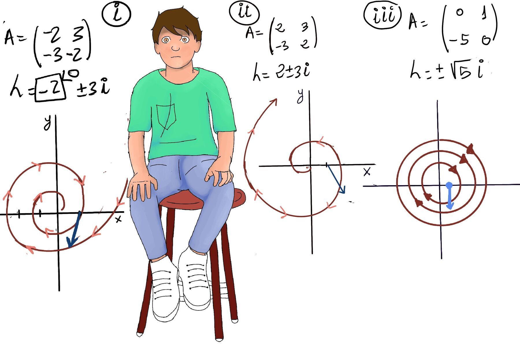
Now let’s examine a system with no real components in its eigenvalues.

$$A = \begin{pmatrix} 0 & 1 \\ -5 & 0 \end{pmatrix}$$

Step 1: Finding the Eigenvalues

We solve the characteristic equation: $\det \begin{pmatrix} -\lambda & 1 \\ -5 & -\lambda \end{pmatrix} = (-\lambda)(-\lambda) - (1)(-5) = \lambda^2 + 5 = 0$

Solving for $\lambda$: $\lambda^2 = -5 \implies \lambda = \pm \sqrt{5}i$

Here, the eigenvalues are purely imaginary. Because there is no real component ($\text{Re}(\lambda) = 0$), there is no exponential growth or decay. The system will neither spiral inward nor outward; instead, it forms closed orbits. This type of equilibrium is known as a center, and the trajectories are ellipses centered at the origin.

Step 2: Finding the Eigenvector for $λ = +\sqrt{5}i$

We solve $(A-\lambda I)\mathbf{v} = 0$: $\begin{pmatrix} -\sqrt{5}i & 1 \\ -5 & -\sqrt{5}i \end{pmatrix} \begin{pmatrix} a_1 \\ a_2 \end{pmatrix} = \begin{pmatrix} 0 \\ 0 \end{pmatrix}$

This gives the system of equations:

1. $-\sqrt{5}i a_1 + a_2 = 0 \implies a_2 = \sqrt{5}i a_1$
2. $-5a_1 - \sqrt{5}i a_2 = 0$

Let $a_1 = 1$, which gives $a_2 = \sqrt{5}i$. The corresponding eigenvector is: $\mathbf{v} = \begin{pmatrix} 1 \\ \sqrt{5}i \end{pmatrix}$

Step 3: Constructing the Complex Solution

Using the eigenvalue and eigenvector, the complex solution is $\mathbf{x}(t) = \mathbf{v} e^{\lambda t}$: $\mathbf{x}(t) = \begin{pmatrix} 1 \\ \sqrt{5}i \end{pmatrix} e^{\sqrt{5}it}$

Applying Euler’s formula ($e^{it} = \cos(t) + i\sin(t)$): $\mathbf{x}(t) = \left[ \begin{pmatrix} 1 \\ 0 \end{pmatrix} + i \begin{pmatrix} 0 \\ \sqrt{5} \end{pmatrix} \right] (\cos(\sqrt{5}t) + i\sin(\sqrt{5}t))$

Step 4: Separating Real and Imaginary Parts to Form Real Solutions

The real and imaginary parts of x(t) give us two linearly independent solutions:

• Real Part: $\mathbf{x}_1(t) = \begin{pmatrix} 1 \\ 0 \end{pmatrix}\cos(\sqrt{5}t) - \begin{pmatrix} 0 \\ \sqrt{5} \end{pmatrix}\sin(\sqrt{5}t) = \begin{pmatrix} \cos(\sqrt{5}t) \\ -\sqrt{5}\sin(\sqrt{5}t) \end{pmatrix}$

• Imaginary Part: $\mathbf{x}_2(t) = \begin{pmatrix} 1 \\ 0 \end{pmatrix}\sin(\sqrt{5}t) + \begin{pmatrix} 0 \\ \sqrt{5} \end{pmatrix}\cos(\sqrt{5}t) = \begin{pmatrix} \sin(\sqrt{5}t) \\ \sqrt{5}\cos(\sqrt{5}t) \end{pmatrix}$

Therefore, the general solution can be written as a linear combination of these two real solutions. The general solution for a system with purely imaginary eigenvalues can be expressed as: $\boxed{\mathbf{x}(t) = C_1 \begin{pmatrix} \cos(\sqrt{5}t) \\ -\sqrt{5}\sin(\sqrt{5}t) \end{pmatrix} + C_2 \begin{pmatrix} \sin(\sqrt{5}t) \\ \sqrt{5}\cos(\sqrt{5}t) \end{pmatrix}}$

Step 5: Interpreting the Solution and Phase Portrait

The eigenvalues are purely imaginary, which indicates that the system has oscillatory behavior and periodic motion, so there is no exponential growth or decay ($\lambda$ has no real part).

The system represents a center, meaning that trajectories will be closed curves (circles or ellipses) around the origin. They neither converge to nor diverge from the origin. Instead, they form closed orbits (Refer to Figure iii for a visual representation and aid in understanding it).

To determine whether the closed trajectories are rotating clockwise or counterclockwise, we examine the effect of A on a standard basis vector $\begin{pmatrix} 1 \\ 0 \end{pmatrix}$: $\begin{pmatrix} 0 & 1 \\ -5 & 0 \end{pmatrix} \begin{pmatrix} 1 \\ 0 \end{pmatrix} = \begin{pmatrix} 0 \\ -5 \end{pmatrix}$

This indicates that a point at $(1,0)$ is pushed directly downwards to $(0,-5)$. This downward pull on the positive x-axis confirms a clockwise rotation around the origin.

Bibliography

1. NPTEL-NOC IITM, Introduction to Galois Theory.
2. Algebra, Second Edition, by Michael Artin.
3. LibreTexts, Calculus and Calculus 3e (Apex). Abstract and Geometric Algebra, Abstract Algebra: Theory and Applications (Judson).
4. Field and Galois Theory, by Patrick Morandi. Springer.
5. Michael Penn, and MathMajor.
6. Contemporary Abstract Algebra, Joseph, A. Gallian.
7. YouTube’s Andrew Misseldine: Calculus. College Algebra and Abstract Algebra.
8. MIT OpenCourseWare [18.03 Differential Equations, Spring 2006], YouTube by MIT OpenCourseWare.
9. Calculus Early Transcendentals: Differential & Multi-Variable Calculus for Social Sciences.