And yet despite the look on my face, you’re still talking and thinking that I care, Anonymous

Recall

Definition. A differential equation is an equation that involves one or more dependent variables, their derivatives with respect to one or more independent variables, and the independent variables themselves, e.g., $\frac{dy}{dx} = 3x +5y, y' + y = 4xcos(2x), \frac{dy}{dx} = x^2y+y, etc.$

It involves (e.g., $\frac{dy}{dx} = 3x +5y$):

Dependent variables: Variables that depend on one or more other variables (y).
Independent variables: Variables upon which the dependent variables depend (x).
Derivatives: Rates at which the dependent variables change with respect to the independent variables, $\frac{dy}{dx}$

Basic linear ODE

In mathematics, a linear ordinary differential equation (ODE) is an equation involving an unknown function and its derivatives, characterized by the property that both the function and its derivatives appear linearly. This means that the unknown function and its derivatives are raised only to the first power. They are never multiplied together, nor are they composed within nonlinear functions (such as $\sin(y)$ or $e^y$). The general form for a first-order linear ODE is: a(x)y’ + b(x)y = c(x).

image info

Second-order Linear Homogeneous ODE’s with Constant Coefficients

In mathematics, a second-order linear homogeneous differential equation ODE with constant coefficients is an equation of the form: ay'' + by' + cy = 0 where:

y(t) is the dependent variable, a function of the independent variable t.
y′ and y′′ are the first and second derivatives of y with respect to t, respectively.
t is the independent variable,
a,b, and c are constant real numbers, with $a \ne 0$.

Alternative definition: a second-order linear homogeneous differential equation (ODE) with constant coefficients is an equation of the form y’’ + Ay’ + By = 0 where A and B are constants.

This equation is characterized by:

Second-Order: The highest derivative present is the second derivative.
Linear: y and its derivatives are all of the first power, and there are no products of y with its derivatives.
Homogeneous: The right-hand side is zero, meaning there are no external forcing functions acting on the system.

This type of differential equation arises frequently in physics and engineering, modeling systems such as mechanical vibrations (mass-spring-damper) and electrical circuits (LRC).

The Principle of General Solution

To solve this ODE, we must find two linearly independent solutions $y_1(t)$ and $y_2(t)$. The fundamental theorem of linear ODEs states that the general solution is a linear combination of these two: $c_1y_1 + c_2y_2$ where c₁ and c₂ are two arbitrary constants determined by initial conditions.

General Solution Method

To find $y_1(t)$ and $y_2(t)$, we assume a solution of the exponential form: y’’ + Ay’ + By = 0, we assume the solution is of the exponential form $y = e^{rt}$ where r is a constant to be determined. The motivation for this assumption is that exponential functions are proportional to their own derivatives, which fits the structure of the ODE.

Substituting or plugging $y = e^{rt}, y'= re^{rt}$ and $y'' = r^2e^{rt}$ into the differential equation gives: $ar^2e^{rt} + bre^{rt} + ce^{rt} = 0$ or $r^2e^{rt} + Are^{rt} + Be^{rt} = 0$ ⇒[Cancelling the common factor $e^{rt}$ (which is never zero), we obtain the characteristic equation:] $ar^2 + br + c = 0$ or $r^2 + Ar + B = 0$.

This is a simple quadratic equation in r. The form of the general solution to the ODE depends on the nature of the roots of this quadratic equation. The nature of the roots leads to three cases:

Distinct Real Roots
Repeated Real Roots
Complex Conjugate Roots

Cases and Physical Examples: The Mass-Spring-Damper Model

To provide physical intuition for the three algebraic cases of the roots, we will use the foundational example of a mechanical mass-spring-damper system

Consider a mechanical system where a mass m is attached to a spring (with spring constant k) and a damper or dashpot (with damping constant c). The mass moves along a vertical x-axis, and its displacement from the equilibrium position at time t is denoted by x(t). The origin of the x-axis is chosen so that the mass’s equilibrium position corresponds to x = 0.

Forces acting on the mass:

Spring Force. Hooke’s law states that the force (restoring force) needed to extend or compress a spring is proportional to the displacement, F_spring = -kx where k is a constant factor characteristic of the spring, the spring’s stiffness.
Damping Force. Provided by the damper, this force cushions movement to avoid shock. It is proportional to the velocity x’: F_damping = -cx’ where c is the damping constant and x’ is the velocity.
A damper is a physical device designed to absorb and dissipate kinetic energy, thereby slowing down or suppressing vibrations, oscillations, and sudden movements.

Newton’s Second Law Applied. The total force acting on the mass is the sum of the spring and damping forces. The movement of the mass is governed by Newton’s second law, which can be written as: $ma = mx'' = F_{total} = F_{spring} + F_{damping} = -kx -cx$ where m is the mass and a is the acceleration (Refer to Figure 1 for a visual representation and aid in understanding it)

Damping forces are a special type of force that are used to slow down or stop a motion. A dashpot is a device for cushioning or damping a movement (as of a mechanical part) to avoid shock.

Undamped and Damped Oscillations

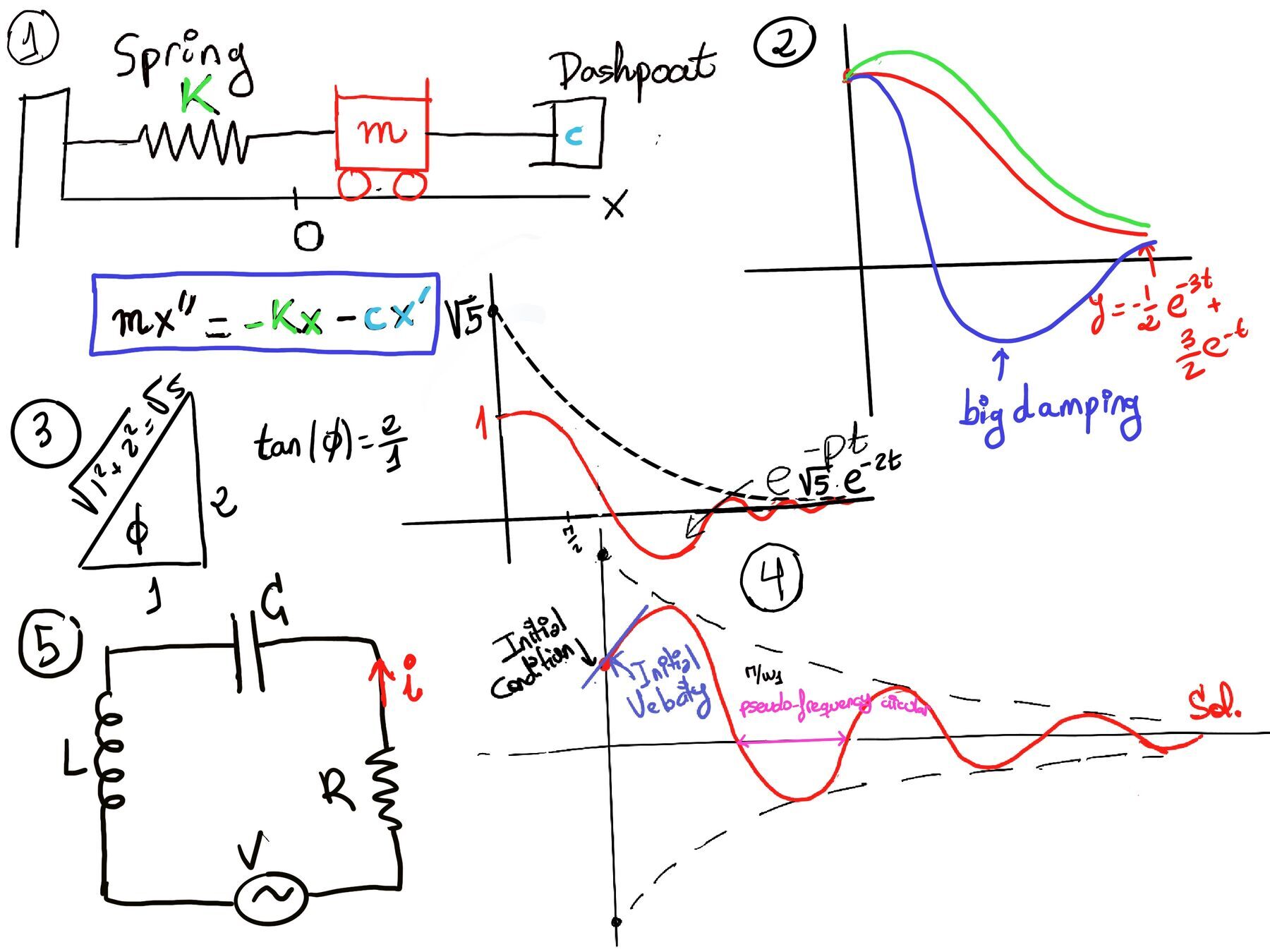
This gives the equation of motion: mx’’ + cx’ + kx = 0 ↭[Dividing both sides by m, we get the simplified or standard form:] $x'' + \frac{c}{m}x'+ \frac{k}{m}x = 0$.

This is a second-order linear homogeneous ODE with constant coefficients. It models the oscillatory motion of the mass-spring-damper system. To solve this equation, we need to find two independent solutions.

The corresponding characteristic equation for this physical system is: $mr^2 + cr + k = 0$

The roots are: $r = \frac{-c \pm \sqrt{c^2 - 4mk}}{2m}$. The three cases for the discriminant ($c^2 - 4mk$) define the physical “damping regimes” of the system

Example: Solving y’’ + 4y’ + 3y = 0

Consider the homogeneous linear ODE: y’’ + 4y’ + 3y = 0. This is a second‑order linear ODE with constant coefficients, so the standard method is to solve its characteristic equation.

Step 1: Write the Characteristic Equation. Replace y with $e^{rt}$. The characteristic equation for the differential equation is: r² + 4r + 3 = 0

Step 2: Solve for the roots. r² + 4y + 3 = 0↭[Factoring gives] (r + 3)(r + 1) = 0. Thus, the roots are r₁ = -3 and r₂ = -1. These are real and distinct, which already tells us the qualitative behavior: the solution is a sum of two decaying exponentials.

Step 3: Write the General Solution. For real, distinct roots $r_1$ and $r_2$, the general solution is: $y(t) = c_1e^{-3t} + c_2e^{-t}$

Substituting our roots: y = $c_1e^{-3t} + c_2e^{-t}$

Step 4: Apply Initial Conditions. Suppose we are given the initial condition y(0) = 1, y’(0) = 0.

To determine c₁ and c₂, we first need to calculate the derivate of y: $y' =-3c_1e^{-3t}- c_2e^{-t} $

Substituting the initial condition t = 0, y(0) = 1: $1 = c_1 + c_2$.

Similarly, substituting y’(0) = 0, $0 = -3c_1 -3c_2$.

Adding both $1 = -2c_1$, so $c_1 = -\frac{1}{2}, c_2 = -3c_1 = \frac{3}{2}$

Step 5: Write the Particular (Final) Solution. The final solution to the differential equation is: $\boxed{y = \frac{-1}{2}e^{-3t} + \frac{3}{2}e^{-t}}$ (Refer to Figure 2 for a visual representation and aid in understanding it). This solution is a weighted combination of two decaying exponentials. The $e^{-t}$ term decays more slowly, so it dominates the long‑term behavior.

Overdamped system

Cases Based on the Roots

Case 1: Real and Distinct Roots (Overdamped System)

When the characteristic equation has two distinct real roots, say $r_1$ and $r_2$, then the general solution is: $\boxed{y = c_1e^{r_1t} + c_2e^{r_2t}}$.

Physical Interpretation (Mechanical/Electrical Systems)

In mechanical or electrical systems, this scenario corresponds to an overdamped system:

The damping is so strong that the system returns to equilibrium without oscillating.
The resistance to motion is so high that the mass slowly creeps back to its equilibrium position (more slowly than if there were no damping) without overshooting.
The terms $e^{r_1t}$ and $e^{r_2t}$ represent two exponentially decaying motions.

Imagine pushing a door through thick mud. It moves back to rest, but sluggishly, and never oscillates. This is exactly what happens in our example: both roots are negative, so both exponentials decay, and the motion is a smooth, non‑oscillatory return to equilibrium.

Case 2. Complex roots (Underdamped System)

A second-order linear homogeneous ODE with constant coefficients has the general form: y′′ + Ay′ +By = 0. To solve this ODE, we assume a solution of the form: y(t) = e^rt. Substituting or plugging $y = e^{rt}$ into the differential equation gives:

$r^2e^{rt} + Are^{rt} + Be^{rt} = 0$ ⇒[Cancelling the common factor $e^{rt}$ (which is never zero), we obtain the characteristic equation:] $r^2 + Ar + B = 0$.

When the characteristic equation of a second-order linear homogeneous ODE with constant coefficients, y′′ + Ay′ + By = 0 has a negative discriminant ($A^2 - 4B \lt 0$), the roots of the equation are complex conjugates.

These roots take the form r = a ± bi, where a and b are real numbers and $b \ne 0$. This case describes an underdamped system in physics, which is characterized by oscillatory behavior where the amplitude of the oscillations gradually decreases over time.

Mathematical Derivation

We get two complex solutions, one of them is $y_{complex}(t) = e^{(a+bi)t} = e^{at}e^{bt i} =[\text{Using Euler's Formula}] e^{at}(cos(bt)+isin(bt))$.

This is a valid complex solution to our ODE. However, to model real-world physical systems, we seek independent real solutions. A key theorem (which we will prove below) states that the real and imaginary parts of any complex solution are themselves real solutions.

Therefore, we can extract our two independent real solutions from $y_{complex}(t)$:

The Real Part: $e^{at}cos(bt)$
The imaginary part: $e^{at}sin(bt)$

The General Solution

A linear combination of these two independent real solutions gives us the general solution for the complex root case.

The general solution to the second-order linear ODE with complex roots is: $y(t) = e^{at}( c_1\cos(bt) + c_2\sin(bt))$ where:

$c_1$ and $c_2$ are arbitrary real constants determined by initial conditions.
$e^{at}$ represents the exponential envelope, which determines whether the oscillations decay (a < 0), grow (a > 0), or maintain a constant amplitude (a = 0).
cos(bt) and sin(bt) represent the oscillatory response with an angular frequency of b.

Polar Representation: Amplitude and Phase

A more physically intuitive way to express this general solution is by using trigonometric identities to combine the sine and cosine terms into a single, phase-shifted oscillation: $\boxed{y(t) = Ce^{at}(cos(bt- Φ))}$ where:

We are using the trigonometry identity a·cos(θ)+b·sin(θ) = c·cos(θ - Φ).
$c = \sqrt{c_1^2+c_2^2}$ is the amplitude constant (the maximum amplitude is $Ce^{at}$).
$\phi = arctan(\frac{c_2}{c_1})$ is the phase angle or phase shift in radians, which shifts the oscillation in time.

Theorem: Real and Imaginary Parts are Solutions

This is a fundamental theorem that allows us to find real solutions from complex ones.

Theorem. If y(t) = u(t) + iv(t) is a complex solution to a second-order linear homogeneous differential equation y'' + Ay' + By = 0 with real coefficients A and B, then both u(t) and v(t) satisfy the differential equation and are real solutions themselves.

Proof.

By assumption u(t) + iv(t) is a solution to a differential equation y’’ + Ay’ + By = 0, substituting into the differential equation: (u + iv)’’ + A(u + iv)’ + B(u + iv) = 0.
Compute derivatives, remember that the derivative of a sum is the sum of the derivatives, and then group the real and imaginary parts, taking into consideration that A and B are real numbers:(u’’ + Au’ + Bu) + (v’’ + Av’ + Bv)i = 0.
Set Real and Imaginary Parts to Zero: For the entire expression on the left to be zero, both the real and imaginary components must be zero. This directly implies: u’’ + Au’ + Bu = 0, v’’ + Av’ + Bv = 0.
Conclusion. This shows that both u(t) and v(t) satisfy the differential equation. Thus, u(t) and v(t) are real-valued solutions to our original ODE.

Worked Example: Damped Oscillations with Specific Initial Conditions

Let’s solve the specific underdamped system y’’ + 4y’ + 5y = 0, given the initial conditions y(0)= 1 and y′(0) = 0.

Step 1: Formulate the Characteristic Equation. The characteristic equation for the differential equation is: r² + 4r + 5 = 0.

Step 2. Solve the Characteristic Equatio. r² + 4r + 5 = 0↭[Using the quadratic formula:] $r = \frac{-4±\sqrt{-4}}{2} = -2±i$. Thus, the roots are: r = -2 ± i. Here, we have a = −2 and b = 1.

Step 3: Write the General Solution. Based on our values of a and b, the general solution is: y = $e^{-2t}(c_1cos(t) + c_2sin(t))$.

Step 4. Apply the initial conditions. Given y(0) = 1, y’(0) = 0.

y(0) = 1 = $e^{0}(c_1cos(0) + c_2sin(0)) = c_1,$ so c₁ = 1.

Next, we we differentiate y(t): $y'(t) = \frac{d}{dt}\left[ e^{-2t} \right] \cdot (c_1\cos(t) + c_2\sin(t)) + e^{-2t} \cdot \frac{d}{dt}\left[ c_1\cos(t) + c_2\sin(t) \right]$

$y'(t) = -2e^{-2t}(c_1\cos(t) + c_2\sin(t)) + e^{-2t}(-c_1\sin(t) + c_2\cos(t))$

Use $y'(0) = 0$ and $c_1 = 1$: Plug in $t=0$ and solve for $c_2$:

$0 = -2e^{0}(c_1\cos(0) + c_2\sin(0)) + e^{0}(-c_1\sin(0) + c_2\cos(0))= -2(1 \cdot 1 + c_2 \cdot 0) + 1(-1 \cdot 0 + c_2 \cdot 1)$

$0 = -2c_1 + c_2 = -2(1) + c_2 \implies c_2 = 2$

Step 5: Write the Unique Particular Solution. The unique particular solution is: $y(t)=e^{-2t}(\cos(t) + 2\sin(t))$

This expression can also be written in its polar form, which provides better insight into the amplitude and phase: $\boxed{y(t) = e^{-2t}(\cos(t) + 2\sin(t)) = \sqrt{5}e^{-2t}\cos(t - \phi)}$ where $c = \sqrt{c_1^2+c_2^2} = \sqrt{1^2+2^2} = \sqrt{5}$ and $\phi$ is a phase angle given by $\phi = arctan(\frac{c_2}{c_1}) = tan^{-1}(\frac{2}{1}) \approx 63.43\deg [\text{or (degrees × π) ÷ 180 = radians}] 1.107$ radians (Refer to Figure 3 for a visual representation and aid in understanding it)