Second-order Linear Homogeneous ODE's. Complex Roots and Damped Oscillations

If the only tool you have is a hammer, you tend to see every problem as a nail, Abraham Maslow.

Recall

Definition. A differential equation is an equation that involves one or more dependent variables, their derivatives with respect to one or more independent variables, and the independent variables themselves, e.g., $\frac{dy}{dx} = 3x +5y, y' + y = 4xcos(2x), \frac{dy}{dx} = x^2y+y, etc.$

It involves (e.g., $\frac{dy}{dx} = 3x +5y$):

• Dependent variables: Variables that depend on one or more other variables (y).
• Independent variables: Variables upon which the dependent variables depend (x).
• Derivatives: Rates at which the dependent variables change with respect to the independent variables, $\frac{dy}{dx}$

Basic linear ODE

In mathematics, a linear ordinary differential equation (ODE) is an equation involving an unknown function and its derivatives, characterized by the property that both the function and its derivatives appear linearly. This means that the unknown function and its derivatives are raised only to the first power. They are never multiplied together, nor are they composed within nonlinear functions (such as $\sin(y)$ or $e^y$). The general form for a first-order linear ODE is: a(x)y’ + b(x)y = c(x).

Second-order Linear Homogeneous ODE’s with Constant Coefficients

In mathematics, a second-order linear homogeneous differential equation ODE with constant coefficients is an equation of the form: ay'' + by' + cy = 0 where:

• y(t) is the dependent variable, a function of the independent variable t.
• y′ and y′′ are the first and second derivatives of y with respect to t, respectively.
• t is the independent variable,
• a,b, and c are constant real numbers, with $a \ne 0$.

This equation is characterized by:

• Second-Order: The highest derivative present is the second derivative.
• Linear: y and its derivatives are all of the first power, and there are no products of y with its derivatives.
• Homogeneous: The right-hand side is zero, meaning there are no external forcing functions acting on the system.

This type of differential equation arises frequently in physics and engineering, modeling systems such as mechanical vibrations (mass-spring-damper) and electrical circuits (LRC).

Complex Characteristic Roots

In the study of second-order linear homogeneous ordinary differential equations (ODEs) with constant coefficients, the nature of the roots of the characteristic equation plays a crucial role in determining the form of the general solution. When the characteristic equation has complex roots, the solutions inherently involve exponential functions combined with sine and cosine functions.

Consider the general second-order linear ODE: y’’ + Ay’ + By = 0. To solve this ODE, we assume a solution of the form: $y = e^{rt}$ where r is a constant to be determined. Substituting or plugging $y = e^{rt}$ into the differential equation, we obtain:

$r^2e^{rt} + Are^{rt} + Be^{rt} = 0$ ⇒[Cancelling the common factor $e^{rt}$ (which is never zero), we obtain the characteristic equation associated with the differential equation:] $r^2 + Ar + B = 0$.

If the discriminant of this quadratic is negative $\Delta = A^2 - 4B \lt 0$, the characteristic equation yields complex roots, which we can write as r = a ± bi.

Deriving the Independent Real Solutions

Using the positive root $r_1 = a + bi$, we get our first complex solution: $y=e^{(a+bi)t} = e^{at}e^{ibt} =[\text{Applying Euler's formula}] e^{at}(cos(bt) + isin(bt)) = e^{at}cos(bt) + ie^{at}sin(bt)$.

From here, we rely on a fundamental theorem: The real and imaginary parts of a complex solution to a linear ODE with real coefficients are themselves valid, independent real solutions.

• Real part: $y_1(t) = e^{at}cos(bt)$.
• Imaginary part: $e^{at}sin(bt)$.

Because $y_1$ and $y_2$ are two linearly independent real solutions, the general solution is their linear combination: $y = c_1y_1 + c_2y_2 = e^{at}(c_1cos(bt)+c_2sin(bt))$

What about the second root ($r_2 = a - bi$)?

If we use the conjugate root, our solution becomes: $y = e^{(a-bi)t} = e^{at}(\cos(-bt) + i\sin(-bt))$

Because cosine is an even function ($\cos(-bt) = \cos(bt)$) and sine is an odd function ($\sin(-bt) = -\sin(bt)$), this simplifies to: $y = e^{at}\cos(bt) - ie^{at}\sin(bt)$

The real part is still $e^{at}\cos(bt)$, and the imaginary part is $-e^{at}\sin(bt)$. Although the sign of $y_2$ change, this does not affect the general solution because the arbitrary constants $c_1$ and $c_2$ simply absorb the negative sign.

Amplitude-Phase Form

Using the trigonometric identity $c_1\cos(\theta) + c_2\sin(\theta) = C\cos(\theta - \Phi)$, we can condense the general solution into a single phase-shifted wave: $\boxed{y(t) = e^{at} \cdot C \cos(bt - \Phi)}$ where the new constants are defined by the initial conditions as:

• Amplitude ($C$): $C = \sqrt{c_1^2 + c_2^2}$

• Phase Shift ($\Phi$): $\Phi = \arctan\left(\frac{c_2}{c_1}\right)$

Alternative Approach Using Complex Constants

Alternatively, we can write the solution directly using the two original complex roots. The general solution is: $y = C_1e^{(a+bi)t}+C_2e^{(a-bi)t}$ where C₁ and C₂ are complex constants.

For $y(t)$ to represent a real physical quantity, the overall imaginary parts of this expression must cancel out. Let’s express $C_1$ and $C_2$ explicitly as complex numbers:

$C_1 = c_1 + id_1$, $C_2 = c_2 + id_2$ (Note: $c_1, c_2, d_1, d_2$ are strictly real numbers, and $i$ is the imaginary unit).

Now, substitute these into the solution and factor out $e^{at}$: $y(t) = e^{at} \left[ (c_1+id_1)e^{ibt} + (c_2+id_2)e^{-ibt} \right]$

Apply Euler’s formula to $e^{ibt}$ and $e^{-ibt}$: $y(t) = e^{at} \left[ (c_1+id_1)(\cos(bt) + i\sin(bt)) + (c_2+id_2)(\cos(bt) - i\sin(bt)) \right]$

Distribute the constants over the trigonometric functions: $y(t) = e^{at} \left[ c_1\cos(bt) + ic_1\sin(bt) + id_1\cos(bt) - d_1\sin(bt) + c_2\cos(bt) - ic_2\sin(bt) + id_2\cos(bt) + d_2\sin(bt) \right]$

Next, carefully group the real terms and the imaginary terms together: $y(t) = e^{at}\left[ (c_1+c_2)\cos(bt) + (d_2-d_1)\sin(bt) \right] + ie^{at}\left[ (c_1-c_2)\sin(bt) + (d_1+d_2)\cos(bt) \right]$

To ensure $y(t)$ is purely real for all values of $t$, the entire imaginary bracket must vanish. This imposes two strict conditions:

1. $c_1 - c_2 = 0 \implies c_1 = c_2$
2. $d_1 + d_2 = 0 \implies d_1 = -d_2$

This elegantly proves that for the solution to be real, $C_1$ and $C_2$ must be complex conjugates. If we let $C_1 = c + id$, then $C_2 = c - id$.

Substituting these back into the real part of the equation yields: $y(t) = e^{at}\left[ (c_1+c_2)\cos(bt) + (d_2-d_1)\sin(bt) \right] = e^{at} \left[ 2c\cos(bt) - 2d\sin(bt) \right]$

If we rename our arbitrary constants ($A = 2c$ and $B = -2d$), we arrive exactly back at the standard general form: $y(t) = e^{at}\left[ A\cos(bt) + B\sin(bt) \right]$. In other words, it exactly matches the general form derived using the typical method Second-order Linear ODE’s with Constant Coefficients.

Physical Significance and Interpretation

In physical systems (such as a mass-spring-damper system or an RLC circuit), complex roots occur when the system is underdamped. This means the restoring force (spring) is strong enough compared to the damping force (friction) that the system overshoots its equilibrium point, resulting in oscillations.

The general solution $y(t) = e^{at}(c_1\cos(bt) + c_2\sin(bt))$ perfectly maps to this physical behavior:

• The Oscillation ($\cos$ and $\sin$): The trigonometric terms dictate the frequency at which the system oscillates back and forth across the equilibrium point. The constant $b$ represents the damped angular frequency.
• The Envelope ($e^{at}$): In stable real-world systems, the constant $a$ is negative. Therefore, $e^{at}$ acts as an exponential decay envelope, gradually squeezing the amplitude of the oscillations down to zero as energy is lost to friction or resistance.

Undamped and Damped Oscillations

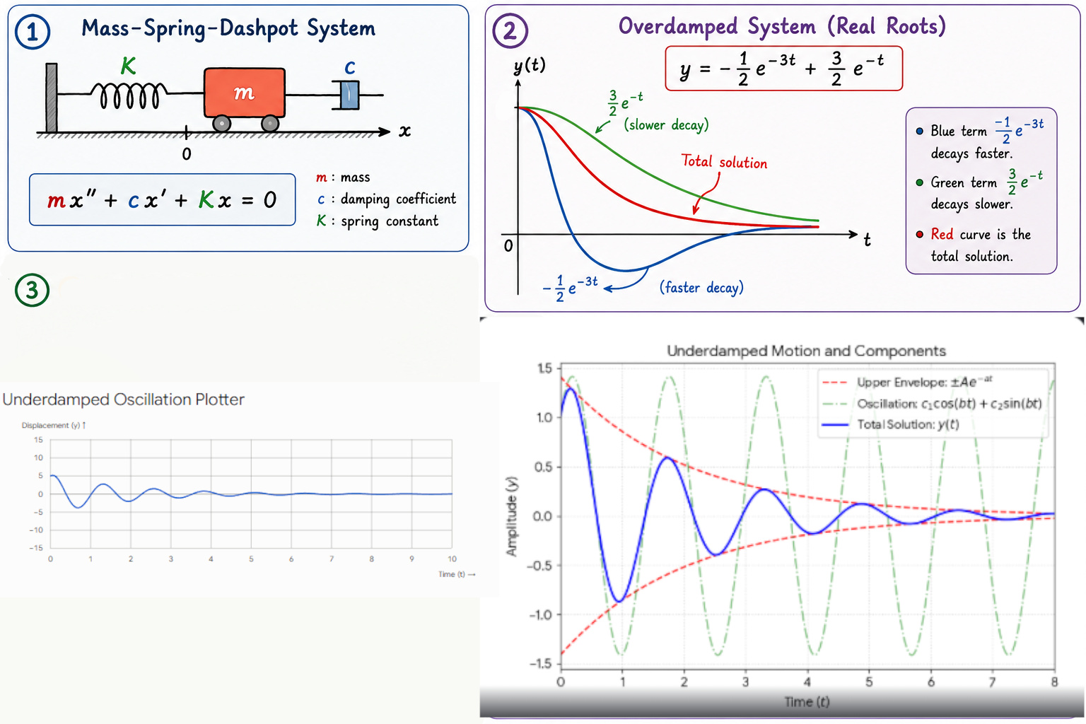
Understanding oscillatory systems is fundamental in maths, physics, and engineering. One of the simplest yet most illustrative models of oscillation is the mass-spring system. This system can exhibit various behaviors depending on parameters such as mass, spring stiffness, and damping. In this explanation, we’ll explore the mathematical modeling of the undamped and damped cases, solve their differential equations, and interpret the physical significance.

Mass-Spring System without Damping

Consider a mass-spring system where a mass m is attached to a spring with a spring constant k. The position of the mass at any time t is denoted by x(t), measured along the x-axis. We choose the origin such that the equilibrium position of the mass corresponds to x = 0. When displaced from equilibrium, the mass oscillates due to the spring’s restoring force.

Newton’s second law states that the sum of forces acting on the mass equals its mass times its acceleration: $F_{\text{total}} = ma = m\frac{d^2x}{dt^2}$

In the undamped case (assuming a vacuum with no friction or air resistance), the only force acting on the mass is the restoring force from the spring, described by Hooke’s Law: $F_{\text{spring}} = -kx$

Hooke’s law states that the force needed to extend or compress a spring by some distance x scales linearly with respect to the displacement distance (in other words, it is proportional to the displacement). The constant k represents the stiffness of the spring. The negative sign indicates that the force always opposes the displacement, aiming to pull or push the mass back to equilibrium.

Setting $F_{\text{total}} = F_{\text{spring}}$ gives us: $m\frac{d^2x}{dt^2}=-kx$.

Dividing by m leads to the standard second-order linear homogeneous ODE for simple harmonic motion: $\frac{d^2x}{dt^2} + \frac{k}{m}x = 0$.

To simplify, we define the natural angular frequency ($\omega_0$) as $\omega_0^2 = \frac{k}{m}$. The equation then becomes: $\boxed{\frac{d^2x}{dt^2} + \omega_0^2x = 0}$

Solution to the Undamped Equation

To solve this, we need to calculate the roots of the characteristic equation: $r^2 + w_0^2 = 0⇒[\text{Solving for r}] r = ± iw_0$.

These are purely imaginary roots, which perfectly correspond to ongoing oscillatory behavior. As established in the rules for second-order linear ODEs with complex roots (r=a±bi), the general solution takes the form: y = $e^{at}(c_1cos(bt)+c_2sin(bt))$

Since our real part $a = 0$ and our imaginary part $b = \omega_0$, the exponential term $e^{0}$ becomes $1$, leaving us with: $x(t) = c_1\cos(\omega_0t) + c_2\sin(\omega_0t)$

Using the trigonometric identity $c_1\cos(\theta) + c_2\sin(\theta) = A\cos(\theta - \Phi)$, we can rewrite this as a single wave: $\boxed{x(t) = A\cos(\omega_0t - \Phi)}$ where:

• $A$ (Amplitude): $A = \sqrt{c_1^2 + c_2^2}$. The maximum displacement from equilibrium.
• $\Phi$ (Phase Shift): $\Phi = \arctan\left(\frac{c_2}{c_1}\right)$.
• $\omega_0$ (Natural Angular Frequency of oscillation): Determines how fast the system oscillates.
• $c_1$ and $c_2$: Arbitrary constants determined by initial conditions (initial position and velocity).

This mathematical solution represents simple harmonic motion, where the system oscillates indefinitely (undamped oscillations) with constant amplitude and frequency.

Inclusion of Damping

In real-world systems, eternal oscillations are impossible; damping can rarely be ignored. Damping refers to the reduction of oscillation amplitude in a system over time due to energy loss. This energy loss occurs for several reasons, including friction between moving parts, air resistance, or intentional dampening devices (like shock absorbers in vehicles).

The damping force ($F_{\text{damping}}$) is typically proportional to the velocity of the mass and directly opposes the direction of motion: $F_{\text{damping}} = -cx' = -c\frac{dx}{dt}$ where:

• $x' = \frac{dx}{dt}$ is the instantaneous velocity.
• c is the damping coefficient, c > 0.

The negative sign indicates opposition to motion.

Total Force and Revised Equation of Motion

The total force on the mass is now the sum of the spring force and the damping force. $F_{\text{total}} = F_{\text{spring}} + F_{\text{damping}} = -kx - c\frac{dx}{dt}$ (Refer to Figure 1 for a visual representation and aid in understanding it).

Applying Newton’s second law ($F_{\text{total}} = m\frac{d^2x}{dt^2}$), we get: $m\frac{d^2x}{dt^2} = -kx -c\frac{dx}{dt}$, we get: $m\frac{d^2x}{dt^2} +c\frac{dx}{dt} + kx = 0$.

Rearranging all terms to one side gives the complete equation of motion: $m\frac{d^2x}{dt^2} + c\frac{dx}{dt} + kx = 0$. This is a second-order linear differential equation that describes exactly how the mass moves over time for a damped mass-spring system.

Standard Form of the Damped Oscillator Equation

To make the math universally applicable, we divide the entire equation by the mass m: $\frac{d^2x}{dt^2} + \frac{c}{m}\frac{dx}{dt} + \frac{k}{m}x = 0$.

By substituting our earlier definition for natural frequency ($\omega_0^2 = \frac{k}{m}$) and introducing a new term for the damping factor ($2\beta = \frac{c}{m}$), the equation is typically expressed in its final, standard form: $\boxed{\frac{d^2x}{dt^2} + 2\beta\frac{dx}{dt} + \omega_0^2x = 0}$ where:

• $2\beta = \frac{c}{m}$ is the damping factor (proportional to the damping coefficient). Damping refers to the process by which energy is lost in an oscillating system, usually due to friction, resistance or dashpots, causing the amplitude of oscillations to decrease over time.

What is a Dashpot? Dashpots are mechanical devices commonly used to purposefully control motion and absorb energy. Everyday examples include shock absorbers in vehicles, door closers (which prevent doors from slamming shut), and dampeners in industrial machinery to reduce vibration and noise in moving parts.

• $\omega_0^2 = \frac{k}{m}$ is the natural angular frequency squared (the inherent oscillation of the system without friction).

Bibliography

1. NPTEL-NOC IITM, Introduction to Galois Theory.
2. Algebra, Second Edition, by Michael Artin.
3. LibreTexts, Calculus and Calculus 3e (Apex). Abstract and Geometric Algebra, Abstract Algebra: Theory and Applications (Judson).
4. Field and Galois Theory, by Patrick Morandi. Springer.
5. Michael Penn, and MathMajor.
6. Contemporary Abstract Algebra, Joseph, A. Gallian.
7. YouTube’s Andrew Misseldine: Calculus. College Algebra and Abstract Algebra.
8. MIT OpenCourseWare [18.03 Differential Equations, Spring 2006], YouTube by MIT OpenCourseWare.
9. Calculus Early Transcendentals: Differential & Multi-Variable Calculus for Social Sciences.