
|
 |

|
|
|
|
|
|
This is your life, and it’s ending one minute at a time, Chuck Palahniuk - Fight Club

A second-order linear homogeneous differential equation ODE with constant coefficients is a differential equation of the form: y'' + Ay' + By = 0, where A and B are constants.
To solve this ODE, we seek two linearly independent solutions $y_1(t)$ and $y_2(t)$. The general solution is then a linear combination of these two solutions: $c_1y_1 + c_2y_2$ where $c_1$ and $c_2$ are two arbitrary constants determined by the system’s initial conditions. The key to finding $y_1$ and $y_2$ is solving the characteristic equation ($r^2 + Ar + B = 0$), whose roots directly determine the behavior of the solutions.
The Exponential Input Theorem provides a direct formula for the particular solution when the forcing term is an exponential function.
Theorem: If $f(x) = e^{\alpha x}$ and $p(\alpha) \neq 0$, the inhomogeneous ODE $p(D)y = e^{\alpha x}$ has a particular solution of the form: $\boxed{y_p = \frac{e^{\alpha x}}{p(\alpha)}}$
We are exploring the phenomenon of resonance through the process of finding particular solutions to second-order linear inhomogeneous differential equations of the form: $y'' + \omega_0^2y = \cos(\omega_1t)$.
This equation perfectly models an undamped system (like a mass on a frictionless spring or an idealized pendulum) that is experiencing an external, periodic forcing, represented by $\cos(\omega_1t)$ where:
The general solution to this inhomogeneous differential equation consists of two parts:
The total response of the system is the sum: $y(t) = y_c(t) + y_p(t)$.
Assuming a solution of the form $y = e^{rt}$, we substitute it into the homogeneous equation: $r^2e^{rt} + \omega_0^2e^{rt} = 0$
Dividing both sides by $e^{rt}$ yields the characteristic equation $r^2 + \omega_0^2 = 0$, which gives purely imaginary roots: $r = \pm i\omega_0$.
Therefore, the complementary solution is: $y_c(t) = c_1\cos(\omega_0t) + c_2\sin(\omega_0t)$ where $c_1$ and $c_2$ are constants determined by initial conditions. This describes the natural, unforced oscillatory behavior of the system with frequency $\omega_0$.
Let’s assume the external push does not match the system’s natural rhythm ($\omega_1 \neq \omega_0$).

Convert the Equation to Differential Operator Form: We rewrite the equation using the differential operator $D = \frac{d}{dt}$: $(D^2 + \omega_0^2)y = \cos(\omega_1t)$
This is a second-order linear inhomogeneous differential equation.
Switch to Complex Exponentials (Easier to Solve): Since working with cosine functions can be tricky and algebraically tedious, we switch to using complex exponentials, as they simplify the process. Using Euler’s formula, we know that: $cos(w_1t)=Re(e^{iw_1t})$
We solve for a complex variable $\tilde{y}$ and take its real part at the end to get our solution for the cosine function.
The equation becomes: $(D^2 + \omega_0^2)\tilde{y} = e^{i\omega_1t}$ where $\tilde{y}$ is the complex solution.
Using the Exponential Input Theorem, if our forcing term is $e^{\alpha t}$, the particular solution is $\tilde{y}_p = \frac{e^{\alpha t}}{p(\alpha)}$, provided the characteristic polynomial evaluated at $\alpha$ is not zero.
In this case, $p(D) = D^2 + \omega_0^2$ and $\alpha = i\omega_1$.
$p(i\omega_1) = (i\omega_1)^2 + \omega_0^2 = -\omega_1^2 + \omega_0^2 = \omega_0^2 - \omega_1^2$
Since by assumption $\omega_1 \neq \omega_0$, we know $p(i\omega_1) \neq 0$. Thus, the complex particular solution is: $\tilde{y}_p = \frac{e^{i\omega_1t}}{\omega_0^2 - \omega_1^2}$
Taking the real part yields our actual particular solution: $\boxed{y_p(t) = \text{Re}(\tilde{y}_p) = \frac{\cos(\omega_1t)}{\omega_0^2 - \omega_1^2}}$
This is the particular solution when the input frequency is not equal to the system’s natural frequency.
If the forcing frequency perfectly matches the natural frequency ($\omega_1 = \omega_0$), we have pure resonance. The previous formula fails because the denominator $\omega_0^2 - \omega_1^2$ becomes zero. We must treat this mathematically in a different way.
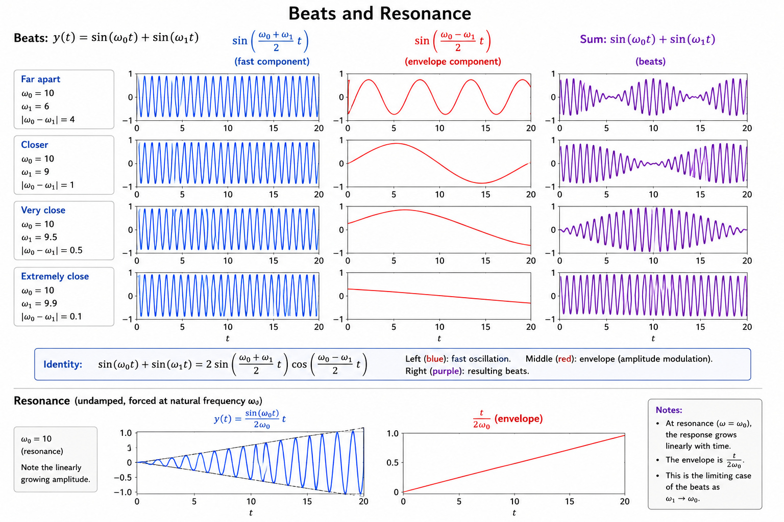
In such cases, the response of the system becomes amplified (the denominator $w_0^2-w_1^2$ get closer to zero, which leads to the amplitude of the response growing significantly), as the forcing frequency aligns with the system’s natural oscillation (Refer to Figure A for a visual representation and aid in understanding it)

We are solving: $(D^2 + \omega_0^2)\tilde{y} = e^{i\omega_0t}$
Again, we convert to complex exponentials $(D^2+w_0^2)\tilde{y} = e^{iw_0t}$.
Because $i\omega_0$ is a root of the characteristic polynomial, we use the modified rule for simple roots: $\tilde{y}_p = \frac{t e^{\alpha t}}{p'(\alpha)}$.
The derivative of our polynomial is $p'(D) = 2D$. Evaluating this at $i\omega_0$ gives $2i\omega_0$.
Therefore, $\tilde{y}_p = \frac{t e^{i\omega_0t}}{2i\omega_0}$
To separate this into real and imaginary parts, recall that $\frac{1}{i} = -i$: $\tilde{y}_p = \frac{-it (\cos(\omega_0t) + i\sin(\omega_0t))}{2\omega_0} = \frac{-it\cos(\omega_0t) + t\sin(\omega_0t)}{2\omega_0}$
Taking the real part gives the particular solution for resonance: $\boxed{y_p(t) = \frac{t\sin(\omega_0t)}{2\omega_0}}$
When $\omega_1 = \omega_0$, the solution has a steadily increasing amplitude. In particular:
If there’s no damping or limit to the oscillation, resonance can cause the amplitude to grow indefinitely, which is why resonance can be both powerful and dangerous (e.g., bridges collapsing due to resonance from wind or traffic)
What happens just before we hit pure resonance? We can discover the resonant solution by taking the non-resonant solution and mathematically forcing $\omega_1 \to \omega_0$.
To avoid dealing with the arbitrary constants in the complementary solution, we can construct a specific particular solution that satisfies initial conditions of rest ($y(0)=0$, $y'(0)=0$).
Start with the General Solution. From our non-resonant case ($\omega_1 \neq \omega_0$), we know the general solution is the sum of the complementary solution and the particular solution: $y(t) = c_1\cos(\omega_0t) + c_2\sin(\omega_0t) + \frac{\cos(\omega_1t)}{\omega_0^2 - \omega_1^2}$
Apply the First Initial Condition ($y(0) = 0$). We know that at $t = 0$, the displacement is zero. Let’s plug $t = 0$ into our general solution:
$y(0) = c_1\cos(0) + c_2\sin(0) + \frac{\cos(0)}{\omega_0^2 - \omega_1^2}$
Since $\cos(0) = 1$ and $\sin(0) = 0$, this simplifies to: $0 = c_1(1) + 0 + \frac{1}{\omega_0^2 - \omega_1^2}$
Now, we just solve for $c_1$: $c_1 = -\frac{1}{\omega_0^2 - \omega_1^2}$
Apply the Second Initial Condition ($y'(0) = 0$).
We know that at $t = 0$, the velocity is zero. First, we need to find the equation for velocity by taking the derivative of our general solution $y(t)$: $y'(t) = \frac{d}{dt} \left[ c_1\cos(\omega_0t) + c_2\sin(\omega_0t) + \frac{\cos(\omega_1t)}{\omega_0^2 - \omega_1^2} \right]$
$y'(t) = -c_1\omega_0\sin(\omega_0t) + c_2\omega_0\cos(\omega_0t) - \frac{\omega_1\sin(\omega_1t)}{\omega_0^2 - \omega_1^2}$
Now, plug in $t = 0$: $y'(0) = -c_1\omega_0\sin(0) + c_2\omega_0\cos(0) - \frac{\omega_1\sin(0)}{\omega_0^2 - \omega_1^2}$
Again, because $\sin(0) = 0$ and $\cos(0) = 1$, the first and third terms completely vanish: $0 = 0 + c_2\omega_0(1) - 0$
$0 = c_2\omega_0$. Since the system’s natural frequency $\omega_0$ is not zero, the only way this equation works is if: $c_2 = 0$
Construct the Final Equation
Now we take our newly discovered constants ($c_1 = -\frac{1}{\omega_0^2 - \omega_1^2}$ and $c_2 = 0$) and substitute them back into the original general solution, and we get: $y(t) = \left( -\frac{1}{\omega_0^2 - \omega_1^2} \right)\cos(\omega_0t) + (0)\sin(\omega_0t) + \frac{\cos(\omega_1t)}{\omega_0^2 - \omega_1^2}$
The sine term disappears entirely. Because the remaining two terms share the exact same denominator, we can combine them into a single fraction: $y(t) = -\frac{\cos(\omega_0t)}{\omega_0^2 - \omega_1^2} + \frac{\cos(\omega_1t)}{\omega_0^2 - \omega_1^2} = \frac{\cos(\omega_1t) - \cos(\omega_0t)}{\omega_0^2 - \omega_1^2}$
If we take the limit as $\omega_1 \to \omega_0$, we get a $\frac{0}{0}$ indeterminate form. We apply L’Hôpital’s Rule, taking the derivative with respect to the variable $\omega_1$: $\lim_{\omega_1 \to \omega_0} \frac{\frac{d}{d\omega_1}[\cos(\omega_1t) - \cos(\omega_0t)]}{\frac{d}{d\omega_1}[\omega_0^2 - \omega_1^2]} = \lim_{\omega_1 \to \omega_0} \frac{-t\sin(\omega_1t)}{-2\omega_1}$
Substituting $\omega_1 = \omega_0$ gives: $\boxed{y(t) = \frac{t\sin(\omega_0t)}{2\omega_0}}$
This result is the particular solution when $\omega_1 = \omega_0$, which corresponds to the resonance case.
When $\omega_1$ is very close to $\omega_0$ (but not exactly equal), the system experiences beats. We can see this by applying a trigonometric sum-to-product identity: $\cos(B) - \cos(A) = 2\sin\left(\frac{A - B}{2}\right)\sin\left(\frac{A + B}{2}\right)$
Applying this to our solution: $y(t) = \frac{\cos(\omega_1t) - \cos(\omega_0t)}{\omega_0^2 - \omega_1^2} = \frac{2\sin\left(\frac{\omega_0 - \omega_1}{2}t\right)\sin\left(\frac{\omega_0 + \omega_1}{2}t\right)}{\omega_0^2 - \omega_1^2}$
This formula reveals two distinct frequencies multiplying each other:
The Fast Oscillation: $\sin\left(\frac{\omega_0 + \omega_1}{2}t\right)$. Because $\omega_1 \approx \omega_0$, this term oscillates rapidly at approximately the system’s natural frequency.
The Slow Envelope (The Beat): $\sin\left(\frac{\omega_0 - \omega_1}{2}t\right)$. Because $\Delta = \omega_0 - \omega_1$ is very small, this creates a slow-moving, long-period wave that dictates the overall amplitude of the fast oscillations.
The envelope frequency is: $\omega_{\text{beat}} = \frac{|\Delta|}{2}$. So the beat period is $T_{\text{beat}} = \frac{2\pi}{\omega_{\text{beat}}} = \frac{4\pi}{|\Delta|} = \frac{4\pi}{|\omega_0 - \omega_1|}$. As $\omega_1 \to \omega_0 \implies |\omega_0 - \omega_1| \to 0, T_{\text{beat}} \to \infty$. The envelope stretches out into a giant, slow swelling wave.
Look at the denominator: $\omega_0^2 - \omega_1^2 = (\omega_0 - \omega_1)(\omega_0 + \omega_1)$. When $\omega_1 \to \omega_0$, then $\omega_0 + \omega_1 \approx 2\omega_0$ (finite), and $\omega_0 - \omega_1 \to 0$. So the denominator shrinks to zero.
Thus, the amplitude: $\frac{1}{|\omega_0^2 - \omega_1^2|}$ blows up. This is the mathematical signature of resonance.
Set $\omega_1 = \omega_0$. Then, the original formula becomes undefined, but the limit exists. We get $y(t) = \frac{\sin(\omega_0 t)}{2\omega_0} t$
A sinusoid multiplied by a linearly growing factor. This is the “infinite beat period” — the envelope becomes a straight line.
To sum up, as $\omega_1$ gets closer and closer to $\omega_0$, the “beat” gets slower and stretches out. The amplitude swells higher and higher. At exact resonance, the beat period becomes infinite, and the amplitude simply grows in a straight line forever. This growth can continue indefinitely in undamped systems, resulting in increasingly large oscillations that may cause structural damage, failure or other dangerous effects.
Why Resonance Matters:

JustToThePoint Copyright © 2011 - 2026 Anawim. ALL RIGHTS RESERVED. Bilingual e-books, articles, and videos to help your child and your entire family succeed, develop a healthy lifestyle, and have a lot of fun. Social Issues, Join us.
This website uses cookies to improve your navigation experience.
By continuing, you are consenting to our
use of cookies, in accordance with our Cookies Policy and
Website Terms and Conditions of use.