Predator-Prey Model (Lotka-Volterra)

As long as algebra is taught in school, there will be prayer in school, Cokie Roberts

Don’t panic, The Hitchhiker’s Guide to the Galaxy

Predator-Prey Model (Lotka-Volterra)

In ecological modeling, predator-prey interactions are crucial for understanding population dynamics within ecosystems. One classic model that describes these interactions is the Lotka-Volterra equations. This model captures the cyclical nature of predator and prey populations, such as sharks (predators) and fish (prey).

Let’s define the variables and parameters:

• a, b, c, d: positive constants representing interaction, death, and growth rates.
• x(t): population of predators (e.g., sharks) at time t.
• y(t): Population of prey (e.g., fish) at time t.

Predator and Prey dynamics

1. Predator Equation ($x'$): In the absence of prey, predators (sharks) die out due to a lack of food, modeled as $x' = -ax$, where $a > 0$ is the natural death rate of predators. However, they experience population growth by consuming prey. This interaction is modeled as $+bxy$, where $b > 0$ represents the rate at which the predator population increases due to successful hunting. $x' = -ax + bxy$
2. Prey Equation ($y'$): Without predators, the prey reproduce and their population grows exponentially: $y' = cy$, where $c > 0$ is the natural growth rate. The prey population decreases as they are consumed by predators, modeled by the interaction term $-dxy$, where $d > 0$ represents the predation rate. $y' = cy - dxy$

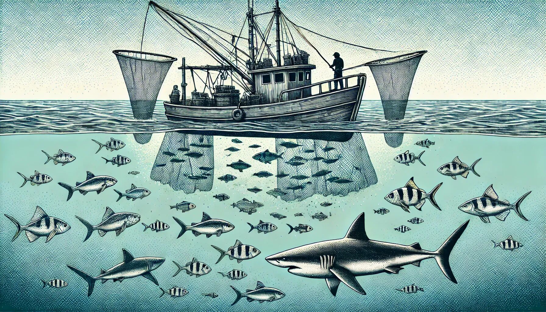
The complete system of non-linear differential equations modeling the interaction is:

$$\begin{cases} x' = x(-a + by) \\ y' = y(c - dx) \end{cases}$$

Finding the Critical Points

Critical points occur where the population sizes do not change over time, meaning $x' = 0$ and $y' = 0$.

Setting the equations to zero gives:

$\begin{cases} x(-a + by) = 0 ~(i)\\\ y(c-dx) = 0 ~(ii)\end{cases}$

• Case 1: If $x = 0$ (no predators), then from equation (ii), $y(c) = 0$. Since $c$ is a positive constant, this forces $y = 0$. This yields the Extinction Equilibrium: $(0, 0)$.
• Case 2: If $x \neq 0$ and $y \neq 0$, then from (i), $-a + by = 0 \implies y = \frac{a}{b}$. From (ii), $c - dx = 0 \implies x = \frac{c}{d}$. This yields the Coexistence Equilibrium: $\left(\frac{c}{d}, \frac{a}{b}\right)$. Both populations are strictly positive here, representing a balanced state where predator and prey can coexist perfectly.

Linearizing the System Near the Origin (0, 0)

To understand what happens near $(0,0)$, we consider very small populations of predators and prey. For very small values of $x$ and $y$, the product terms $bxy$ and $dxy$ become infinitesimally small and are negligible compared to the linear terms $-ax$ and $cy$.

Linearized System at (0,0):

$$\begin{cases} x' = -ax \\ y' = cy \end{cases}$$

Matrix Representation: $\begin{pmatrix} x' \\ y' \end{pmatrix} = \begin{pmatrix} -a & 0 \\ 0 & c \end{pmatrix} \begin{pmatrix} x \\ y \end{pmatrix}$

If we have a diagonal matrix, the eigenvalues are simply the diagonal elements. Therefore, $\lambda_1 = -a$ (which is negative since $a > 0$), and $\lambda_2 = c$ (which is positive since $c > 0$).

The general solution near the origin is decoupled: $\boxed{x(t) = x_0 e^{-at}, \quad y(t) = y_0 e^{ct}}$

• Negative Eigenvalue ($\lambda_1 = -a < 0$): Corresponds to a stable direction along the $x$-axis (predator population). Solutions decay exponentially toward zero. Biological meaning: The predator population rapidly decreases to zero if there are no prey.

• Positive Eigenvalue ($\lambda_2 = c > 0$): Corresponds to an unstable direction along the $y$-axis (prey population). Solutions grow exponentially. Biological meaning: The prey population explodes in the absence of predators.

Since one eigenvalue is strictly negative and the other is strictly positive, the critical point (0,0) is a saddle point. Saddle points are unstable because trajectories move toward the critical point along the stable direction (predators dying out) and shoot away from it along the unstable direction (prey multiplying out of control).

Simplifying the Model for Coexistence

To cleanly analyze the coexistence equilibrium, let’s simplify the model by assuming $a = b = c = d = 1$. The system becomes:

$$\begin{cases} x' = -x + xy \\ y' = y - xy \end{cases}$$

Critical points with simplified parameters: $(0, 0)$ and $(1, 1)$.

Linearizing at the Non-Zero Critical Point (1, 1)

To linearize the system at the coexistence critical point $(1, 1)$, we calculate the Jacobian matrix: $J(x,y) = \begin{pmatrix} \frac{\partial x'}{\partial x} & \frac{\partial x'}{\partial y} \\ \frac{\partial y'}{\partial x} & \frac{\partial y'}{\partial y} \end{pmatrix} = \begin{pmatrix} -1+y & x \\ -y & 1-x \end{pmatrix}$

Evaluate at (1, 1): $(\begin{smallmatrix}-1+y & x\\\ -y & 1-x\end{smallmatrix})\bigg|_{(1, 1)} = (\begin{smallmatrix}0 & 1\\\ -1 & 0\end{smallmatrix})$.

The linearized system locally behaves as:

$$\begin{cases} x' = y \\ y' = -x \end{cases}$$

Deriving the Second-Order ODE: Differentiating the first equation with respect to $t$ yields $x'' = y'$. Substituting $y'$ from the second equation gives $x'' = -x$, or $x'' + x = 0$. This is the classic equation for a simple harmonic oscillator.

The characteristic equation is obtained from $\det(J - \lambda I) = 0$: $\det \begin{pmatrix} -\lambda & 1 \\ -1 & -\lambda \end{pmatrix} = \lambda^2 + 1 = 0 \implies \lambda = \pm i$

The eigenvalues are purely imaginary ($\alpha = 0, \beta = 1$).

The general solution to this linearized system is: $\boxed{\begin{pmatrix} x(t) \\ y(t) \end{pmatrix} = C_1 \begin{pmatrix} \cos(t) \\ -\sin(t) \end{pmatrix} + C_2 \begin{pmatrix} \sin(t) \\ \cos(t) \end{pmatrix}}$

The general solution to this system $\lambda = \alpha \pm \beta i$ is $x(t) = e^{\alpha t}[C_1(\begin{smallmatrix}\cos(\beta t)\\\ -\sin(\beta t)\end{smallmatrix})+ C_2(\begin{smallmatrix}sin(\beta t)\\\ cos(\beta t)\end{smallmatrix})]$

Both $x(t)$ and $y(t)$ rely purely on sine and cosine functions. Because there is no real part in the eigenvalues ($\alpha = 0$), there is no exponential growth or decay. The solutions are strictly periodic with a constant amplitude. Plotting $x(t)$ versus $y(t)$ yields closed concentric circles around $(1,1)$.

At $(1, 1)$, the trajectories represent continuous, sustained oscillations of predator and prey populations around their equilibrium values. Populations perpetually return to their exact starting values after each cycle.

Trace-Determinant Analysis and Structural Stability

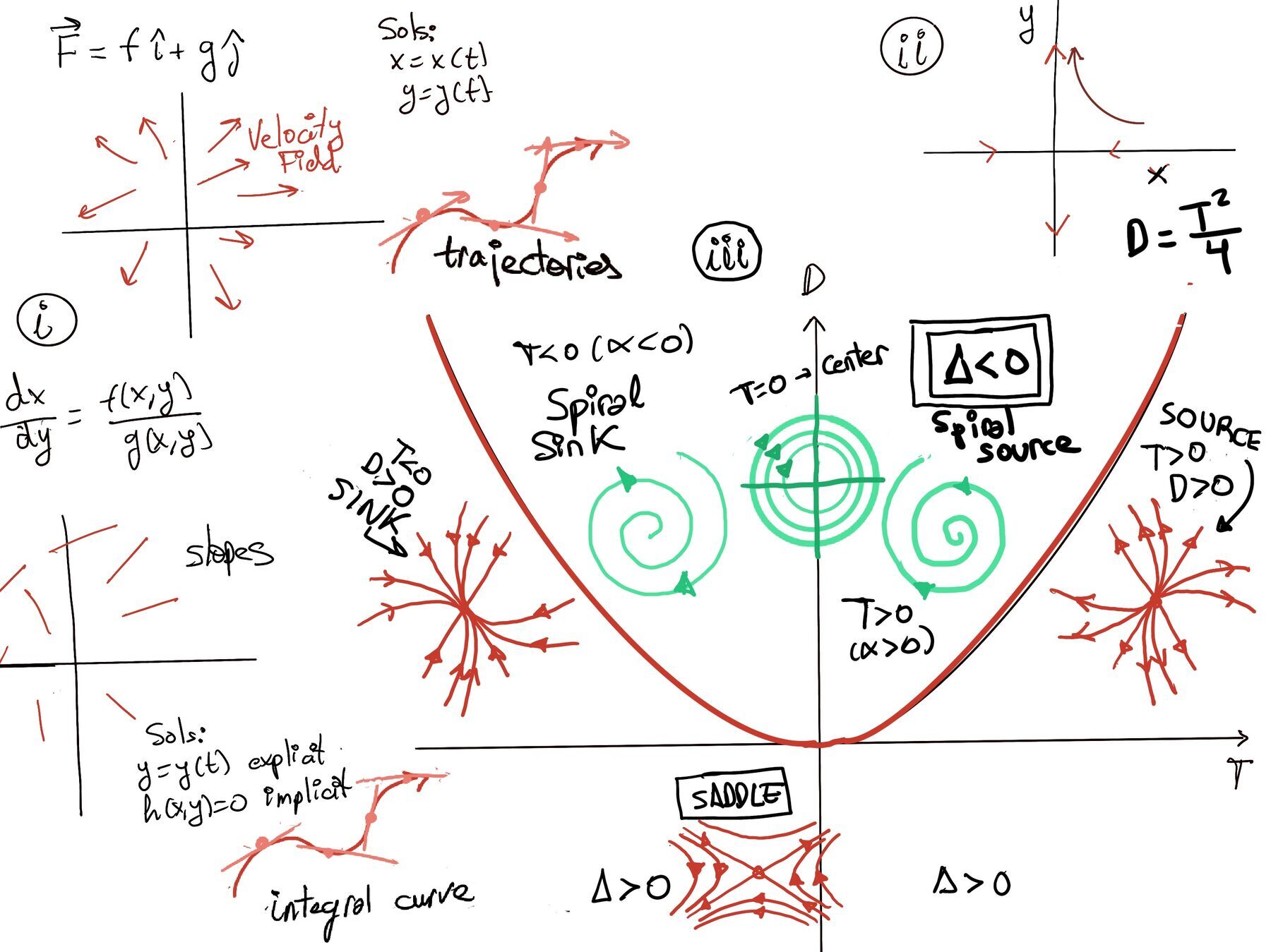
Let’s apply the Trace-Determinant classification to the Jacobian at $(1,1)$: $J = \begin{pmatrix} 0 & 1 \\ -1 & 0 \end{pmatrix}$

• Characteristic Equation: $\lambda^2 -T \lambda + D = 0$ where T is the trace Trace (sum of diagonal elements) and D is the determinant of the Jacobian matrix.
• Trace ($T$): $0 + 0 = 0$
• Determinant ($D$): $(0)(0) - (1)(-1) = 1$
• Discriminant ($\Delta$): $T^2 - 4D = 0^2 - 4(1) = -4$

Interpretation:

• A negative discriminant ($\Delta = -4$) guarantees complex eigenvalues.
• Centers Lie Along $T = 0$. Because $T=0$, the real part of the eigenvalues ($\frac{T}{2}$) is zero. This corresponds to a center, which is neutrally stable. The system does not attract or repel trajectories but keeps them orbiting indefinitely.

The Fragility of Centers (Structural Instability)

In dynamical systems theory, centers are known to be structurally unstable. They lie exactly on the razor’s edge ($T=0$) between stable spirals ($T < 0$) and unstable spirals ($T > 0$).

Because linearization is only an approximation of a non-linear system, the non-linear terms we ignored can sometimes act like a tiny “hidden trace” that destroys the center.

• If a small parameter change makes the trace positive (T > 0), the equilibrium would become a spiral source (unstable focus), as eigenvalues gain a positive real part.
• If a small parameter change makes the trace negative (T < 0), the equilibrium would become a spiral sink (stable focus), as eigenvalues gain a negative real part.

The linearized system at (1, 1) exhibits center behavior, but in many real-world systems, non-linearities or small parameter changes dictate whether it acts as a true center, a spiral sink, or a spiral source.

Why does the standard Lotka-Volterra model maintain perfect centers? Miraculously, the pure Lotka-Volterra equations form an exception to this fragility. The non-linear system actually possesses a conserved quantity (similar to the conservation of energy in physics), ensuring that trajectories remain perfectly closed. However, if you add even a tiny bit of biological realism to the model —such as a carrying capacity for the prey (logistic growth)— the delicate center collapses instantly into a stable spiral sink, causing the populations to eventually settle at a static coexistence rather than oscillating forever.

Another approach: Eliminating time to find trajectories

In a two-dimensional autonomous system such as the Lotka-Volterra model, we are often interested in the geometry of the trajectories —the path traced by the state $(x,y)$— rather than the explicit time-evolution of the populations.

Given the system: $\begin{cases} x' = -ax + bxy ~(i)\\\ y' = cy -dxy ~(ii)\end{cases}$

To find the trajectories, we eliminate $t$ by taking the ratio of the two equations: $\frac{dy}{dx} = \frac{y'}{x'} = \frac{y(1-x)}{x(y-1)}$

Separating the variables $x$ and $y$: $\frac{y-1}{y} \, dy = \frac{1-x}{x} \, dx \implies \left(1 - \frac{1}{y}\right) dy = \left(\frac{1}{x} - 1\right) dx$

Integration and Conserved Quantities

Integrating both sides: $\int \left(1 - \frac{1}{y}\right) dy = \int \left(\frac{1}{x} - 1\right) dx$

$y - \ln(y) = \ln(x) - x + C_1$

Rearranging to group terms involving $x$ and $y$: $x - \ln(x) + y - \ln(y) = C_1 \implies \ln(x) - x + \ln(y) - y = -C_1$

Exponentiating both sides results in a conserved quantity $h(x, y)$: $e^{\ln(x) - x + \ln(y) - y} = e^{-C_1} \implies x e^{-x} \cdot y e^{-y} = C$. The integral curves (trajectories of the system) are graphs of this equation. These are contour curves of $xe^{-x}·ye^{-y} = h(x, y)$ (h is constant along any trajectory).

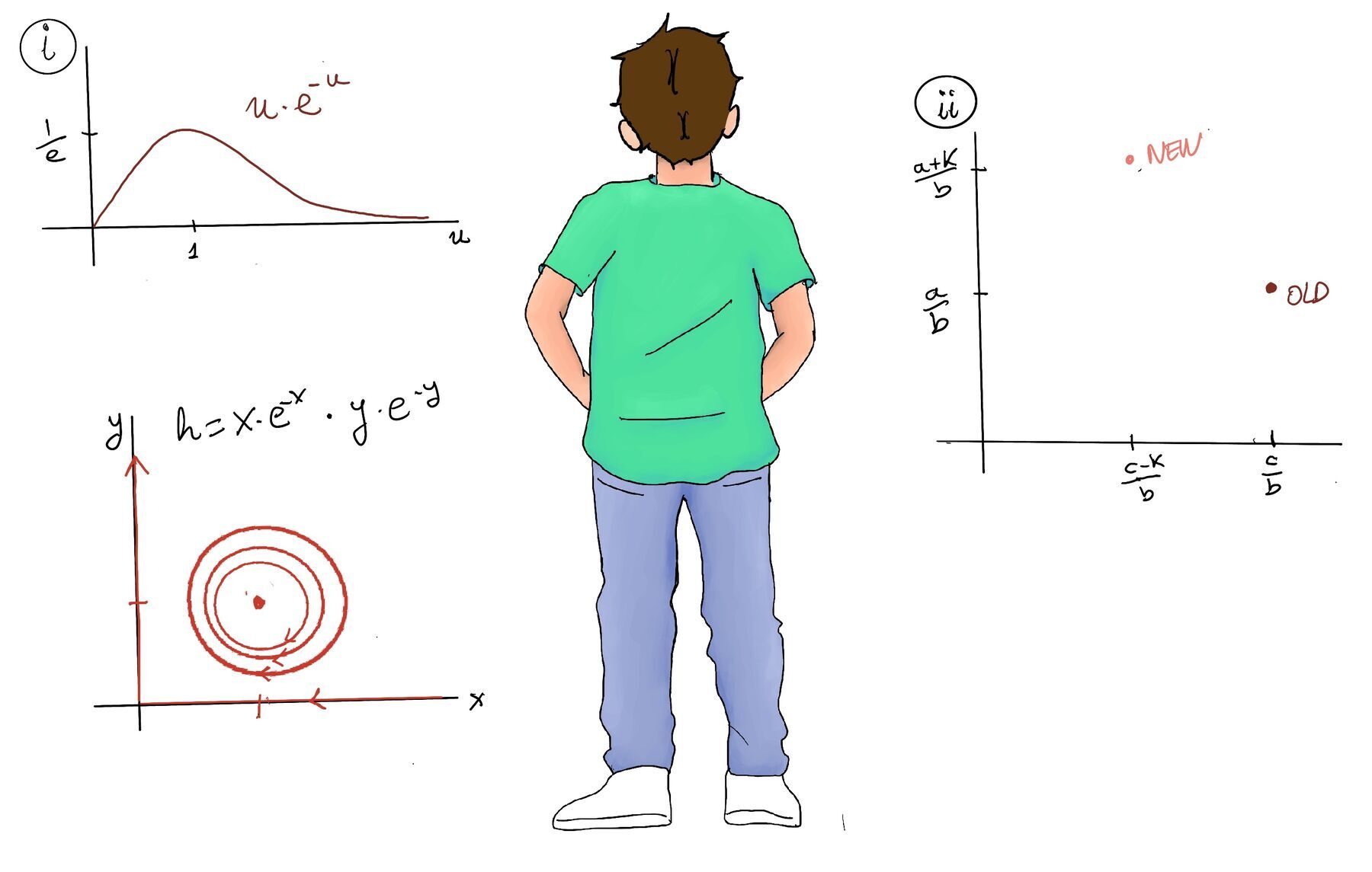
Consider the function $f(u) = ue^{-u}$. This function reaches its maximum at 1 where $f(1)=\frac{1}{e}$. Similarly, $ve^{-v}$ has a maximum at 1, too. h(x, y) is the product of both functions, h(x, y) = f(x)·f(y), hence h(x, y) has a maximum at (1, 1). At (1, 1), the value is $h(1, 1) = (\frac{1}{e})^2$, that is, as a figure of speech, the peak of the mountain.

As we move away from (1, 1), either by letting x or y go to 0 or approach infinity, h(x,y) tends to zero. Thus, the level set (contour curves) h(x, y) = $xe^{-x}·ye^{-y} = C$ formed closed curves around (1, 1). These are concentric closed curves that move clockwise around (1, 1). These represent the closed orbits in the phase plane, confirming the oscillatory behavior of the system (populations oscillate around the equilibrium point (1, 1)).

Biological Interpretation of the Trajectories

The level sets of $h(x, y) = C$ define the path of the populations:

1. High Predator, Low Prey: When predator numbers (x) are high and prey (y) are low, predators quickly consume the remaining prey. Prey population declines further due to intense predation. Eventually, with not enough prey to sustain them, predators also decline.
2. Low Predator, High Prey: If predator numbers are low, predation pressure is reduced. The prey population can grow more easily because fewer are eaten. This increase in prey, in turn, supports a recovery in the predator population since there is now more food available.
3. Repeatedly cycling through these scenarios leads to an endless cycle of population rises and falls. The system’s dynamics reflects natural population oscillations observed in predator-prey relationships. The system’s dynamics show that neither population settles to a constant nonzero value; instead, they oscillate around the equilibrium.

External Factors: Volterra’s Principle

Now consider modifying the system to include an external harvesting (fishing with nets or pesticide use) at a constant rate k.

The system transforms:

$\begin{cases} x' = -ax + bxy -kx ~(i)\\\ y' = cy -dxy -ky ~(ii)\end{cases}$ where the terms −kx and -ky represents additional deaths due to fishing.

Combining terms:

$\begin{cases} x' = -(a+k)x + bxy ~(i)\\\ y' = (c-k)y -dxy ~(ii)\end{cases}$

The Shift in Equilibrium

1. From $x′ = 0: -(a+k)x + bxy = 0 \implies x[−(a+k)+by] = 0 \implies x = 0$ or y = $\frac{a+k}{b}$
2. From $y' = 0: cy -dxy -ky = 0 \implies y[(c−k)−dx] = 0 \implies y = 0$ or x = $\frac{c-k}{d}$

Solving for $x' = 0$ and $y' = 0$ reveals the new equilibrium point: $\left(x^*, y^*\right) = \left(\frac{c-k}{d}, \frac{a+k}{b}\right)$

Compare this to the original equilibrium $(\frac{c}{d}, \frac{a}{b})$. The critical point shifts to: $(\frac{c-k}{d}, \frac{a+k}{b})$ (Refer to Figure ii for a visual representation and aid in understanding it).

Effect on Populations:

• Predator Population (x) Decreases: Since c -k < c (because k > 0) ↭ $x = \frac{c-k}{d} < \frac{c}{d}$, so x decreases. Predator population at equilibrium decreases.
• Prey Population (y) Increases: Since a + k > a ↭ $\frac{a+k}{b} > \frac{a}{b}$, so y increases. This shift reflects the decrease in predators and increase in prey.

The Paradox of Intervention

This result is counterintuitive but mathematically robust. Volterra’s Principle states that if both predator and prey are subjected to proportional mortality (e.g., fishing with nests), the prey population (fish) increases on average, while the predator population (shark) decreases.

Fishing removes prey and predators directly (-ky, -kx). Reduced predator numbers lead to fewer prey being eaten. The indirect positive effect outweighs the direct negative effect, resulting in a higher prey and lower predator population at equilibrium.

Statement of Volterra’s Principle: If both predator and prey populations are subjected to a proportional external mortality (e.g., fishing, pollution, pesticides, etc.) that affects them equally, the prey population will increase on average, while the predator population will decrease on average.

The Lotka-Volterra equations provide valuable insights into predator-prey dynamics, demonstrating how interactions between species can lead to oscillatory behaviors. By analyzing the system’s critical points, linearizing near these points, and understanding the effects of external factors like fishing, we gain a deeper appreciation for the complex balance within ecosystems.

Analogy: Mosquito Plague and Pesticides

Suppose a fish pond experiences a mosquito infestation. What should we do? Let’s assume that the decision is to spray pesticides (e.g., DDT) to kill those pesky mosquitoes. This is a common ecological intervention - the application of pesticides to control a “pest” (the prey). However, the Lotka-Volterra model demonstrates why this can be counterproductive:

Unintended Consequences. The result is quite the same as before because:

1. Pesticides harm both mosquitoes and fish. Non-Selective Impact. When pesticides are applied, they do not discriminate between target and non-target species. Pesticides often affect both mosquitoes and their natural predators (like fish or dragonflies), leading to unintended mortality in fish populations.
2. Fish are natural predators of mosquitoes. Reduced Natural Control. Fish help control mosquito populations by preying on their larvae. Reducing the fish population diminishes this natural control mechanism (“top-down” pressure that keeps the prey in check).
3. Reducing the fish population can lead to a mosquito population increase due to reduced predation. The Rebound With fewer fish to consume mosquito larvae, mosquito numbers can rebound or even increase, exacerbating the original infestation problem.

Careful analysis and consideration of ecological interactions are essential for sustainable management.

Bibliography

1. NPTEL-NOC IITM, Introduction to Galois Theory.
2. Algebra, Second Edition, by Michael Artin.
3. LibreTexts, Calculus and Calculus 3e (Apex). Abstract and Geometric Algebra, Abstract Algebra: Theory and Applications (Judson).
4. Field and Galois Theory, by Patrick Morandi. Springer.
5. Michael Penn, and MathMajor.
6. Contemporary Abstract Algebra, Joseph, A. Gallian.
7. YouTube’s Andrew Misseldine: Calculus. College Algebra and Abstract Algebra.
8. MIT OpenCourseWare [18.03 Differential Equations, Spring 2006], YouTube by MIT OpenCourseWare.
9. Calculus Early Transcendentals: Differential & Multi-Variable Calculus for Social Sciences.