Non-linear Autonomous Systems. Predator-Prey Analysi

If you hear a voice within you say ‘you cannot paint’, then by all means paint and that voice will be silenced, Vincent van Gogh

Recall

Analyzing non-linear autonomous systems like the lightly damped pendulum involves:

• Identifying critical points where the system is in equilibrium.
• Linearizing the system near these points using the Jacobian matrix to approximate behavior.
• Calculating eigenvalues and eigenvectors to determine stability and dynamics (e.g., sinks, saddles, nodes).
• Interpreting physical behavior in terms of the mathematical results.
• Sketching phase portraits to visualize the system’s global trajectories and gain insight into complex behaviors that non-linear systems can exhibit, such as oscillations, damping, and instability.

Predator-Prey System Analysis

In ecological modeling, predator-prey systems are critical tools for understanding the interactions between two species: one being the prey and the other the predator. These models help researchers predict population dynamics and can assist and inform policymakers and conservationist to design and implement conservation and management strategies.

Consider the following system of differential equations: $\begin{cases} x' = x(3-x)-xy \\\ y' = y(1-y) + xy \end{cases}$ where:

• x(t) represents the prey population at time t.
• y(t) represents the predator population at time t.
• The term x(3−x) in the x’ equation is a logistic growth term for the prey. Without predators, the prey population grows but has a carrying capacity of 3.
• Similarly, The term y(1−y) in the y’ equation is a logistic growth term for the predators. Without prey, predators also have a logistic growth with a carrying capacity of 1.
• The term -xy in x′ represents the decrease in prey due to predation. The presence of predators (y) reduces the prey population growth.
• The term +xy in y′ represents the increase in predators (how the predator population increase) due to consuming prey.
• Without the interaction term xy, both populations would exhibit isolated logistic growth: The prey has a carrying capacity of 3. The predator has a carrying capacity of 1 🚀.

🚀 Definition: The carrying capacity is the maximum population size of species that an environment can sustain indefinitely, given the availability of resources such as food, habitat, water, and other environmental conditions.

It is commonly denoted by K in population models. It represents the equilibrium point where the population stabilizes due to resources becoming limited, alongside other limiting factors like competition, predation (when considering prey-predator interactions), disease, and waste accumulation, slowing down growth. Eventually, the population stabilizes at K, where growth stops because births and deaths balance out.

The logistic growth equation models how a population grows rapidly at first and then slows as it approaches the carrying capacity. For a population N(t): $\boxed{N' = rN(1-\frac{N}{K})}$ where

• N(t) is the population at time t; r is the intrinsic growth rate; K is the carrying capacity; and N′ is the rate of change of the population.
• Initial Exponential Growth: When N is much less than K (N « K), the term $(1-\frac{N}{K})≈1$, so the population grows exponentially.
• Growth Rate Decreases: As N approaches K, $(1-\frac{N}{K})$ decreases, slowing the growth.
• Stabilization: The population stabilizes at N = K, where growth stops (N′ = 0).

Application to the Prey-Predator Model

1. Prey Equation. $x′ = x(3 − x) = 3x(1-\frac{x}{3})$. This is a logistic growth equation. Growth rate and carrying capacity: r = K = 3. The prey population will grow until it reaches a maximum sustainable size of 3 units (thousands, millions, etc., depending on the context).
2. Predator Equation: $y′ = y(1 − y)$. This is also a logistic growth equation. Carrying Capacity: K = 1. The predator population will grow until it approaches a maximum sustainable size of 1 unit.

Step-by-Step Analysis

Step 1: Finding the Critical Points

Critical points occur where the populations do not change over time, i.e., where x′ = 0 and y′= 0, meaning neither population is changing at that instant.

$x' = x(3-x) - xy = 0 \implies x = 0 \text{ or } x(3-x) = xy \iff y = 3 - x$

$y' = y(1-y) + xy = 0 \implies y = 0 \text{ or } y(1-y) = -xy \iff x = y - 1$

Therefore, the critical points are:

• $(0, 0)$
• $x = 0, y = x + 1 \implies$ $(0, 1)$
• $y = 0, x = 3 - y \implies$ $(3, 0)$
• $y = 3 - x, x = y - 1 = 3 - x - 1 = 2 - x \iff 2x = 2 \iff x = 1, y = 2 \implies$ $(1, 2)$

Step 2: Linearizing the System Near Each Critical Point.

To understand how the system behaves near these equilibrium points, we use linearization. This involves finding the Jacobian matrix, which is the matrix of first-order partial derivatives of the system.

The Jacobian matrix $J(x,y)$ is: $J(x, y) = \begin{pmatrix} \frac{\partial f}{\partial x} & \frac{\partial f}{\partial y} \\ \frac{\partial g}{\partial x} & \frac{\partial g}{\partial y} \end{pmatrix}$, where: $f(x, y) = x(3-x) - xy = 3x - x^2 - xy$ and $g(x,y) = y(1-y) + xy = y - y^2 + xy$.

$J(x, y) = \begin{pmatrix} 3-2x-y & -x \\ y & 1-2y+x \end{pmatrix}$

Step 3: Evaluating the Jacobian at Each Critical Point

$J(0, 0) = \begin{pmatrix} 3-0-0 & -0 \\ 0 & 1-0+0 \end{pmatrix} = \begin{pmatrix} 3 & 0 \\ 0 & 1 \end{pmatrix}$

J(0, 1) = $(\begin{smallmatrix}3−0−1 & −0\\\ 1 & 1−2⋅1+0\end{smallmatrix}) = (\begin{smallmatrix}2 & 0\\\ 1 & -1\end{smallmatrix})$

J(3, 0) = $(\begin{smallmatrix}3−2⋅3−0 & −3\\\ 0 & 1−0+3\end{smallmatrix}) = (\begin{smallmatrix}-3 & -3\\\ 0 & 4\end{smallmatrix})$

J(1, 2) = $(\begin{smallmatrix}3−2⋅1−2 & −1\\\ 2 & 1−2⋅2+1\end{smallmatrix}) = (\begin{smallmatrix}-1 & -1\\\ 2 & -2\end{smallmatrix})$

Step 4: Computing Eigenvalues and Eigenvectors

We determine the stability of each critical point by finding the eigenvalues of the Jacobian matrices at those points. The sign of the real parts of the eigenvalues tells us if the equilibrium is stable (eigenvalues have negative real parts) or unstable (at least one eigenvalue has a positive real part).

• The Origin. J(0, 0) = $(\begin{smallmatrix}3 & 0\\\ 0 & 1\end{smallmatrix})$. Characteristic equation: $(3-\lambda)(1-\lambda) = 0.$ Eigenvalues: $\lambda_1 = 3$, $\lambda_2 = 1$.

Computing Eigenvectors. We solve $(J-λI)\vec{v} = \vec{0}$ for each eigenvalue.

For $\lambda_1 = 3$: $(\begin{smallmatrix}0 & 0\\\ 0 & -2\end{smallmatrix})(\begin{smallmatrix}a_1\\\ a_2\end{smallmatrix})$. Equation $-2a_2 = 0⇒ a_2 = 0,\text{Eigenvector: } \vec{v_1} = (\begin{smallmatrix}1\\\ 0\end{smallmatrix})$ (x-axis direction)

For $\lambda_2 = 1$ $(\begin{smallmatrix}2 & 0\\\ 0 & 0\end{smallmatrix})(\begin{smallmatrix}a_1\\\ a_2\end{smallmatrix})$. Equation $2a_1 = 0⇒ a_1 = 0,\text{Eigenvector: } \vec{v_2} = (\begin{smallmatrix}0\\\ 1\end{smallmatrix})$ (y-axis direction)

Both eigenvalues are positive, indicating that any small perturbation will cause the system to move away from this point. Trajectories move away from (0, 0) along the x-axis and y-axis. This is not a stable state; any small introduction of individuals (prey or predators) leads to population growth. This equilibrium is an unstable node.

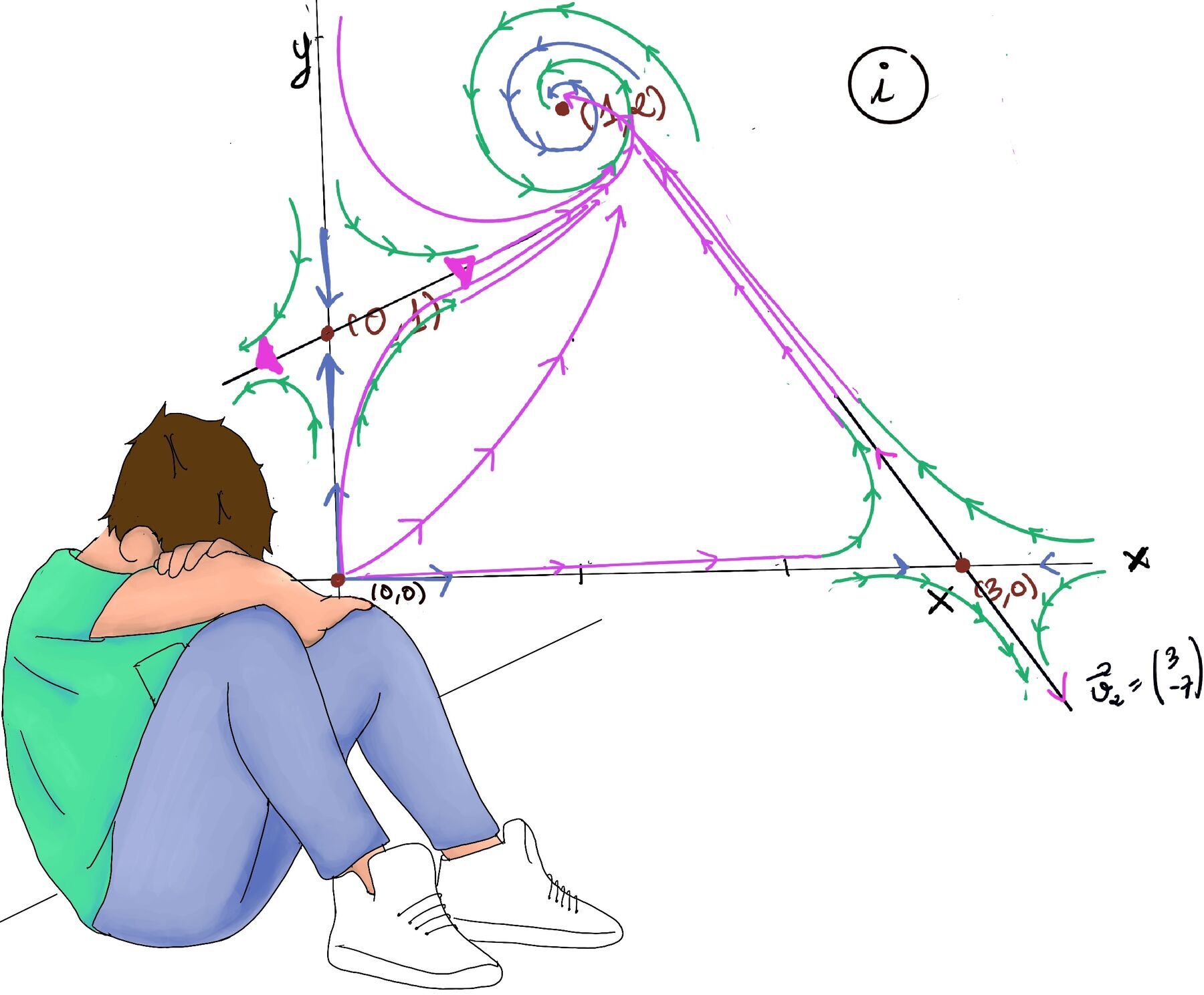
Biological Meaning: If both populations are near zero, they will grow rapidly away from zero. Neither species remains extinct; they tend to increase from this point. Refer to Figure i for a visual representation and aid in understanding it.

• Predators Only. $J(0, 1) = \begin{pmatrix} 3-0-1 & -0 \\ 1 & 1-2(1)+0 \end{pmatrix} = \begin{pmatrix} 2 & 0 \\ 1 & -1 \end{pmatrix}$.

Characteristic Equation: $(2-\lambda)(-1-\lambda) = 0 \implies$ Eigenvalues: $\lambda_1 = 2, \lambda_2 = -1$.

Eigenvectors:

• For $\lambda_1 = 2, (\begin{smallmatrix}0 & 0\\\ 1 & -3\end{smallmatrix})(\begin{smallmatrix}a_1\\\ a_2\end{smallmatrix})$. Equation $a_1-3a_2 = 0 \implies a_1 = 3a_2,\text{Eigenvector: } \vec{v_1} = (\begin{smallmatrix}3\\\ 1\end{smallmatrix})$ (Unstable direction).

$(x, y) = (0, 1) + t(3, 1); x = 3t, y = 1 + t;$ In Cartesian form: $y -1 = \frac{1}{3}x \implies y = 1 + \frac{x}{3}$.

• For $\lambda_2 = -1, (\begin{smallmatrix}3 & 0\\\ 1 & 0\end{smallmatrix})(\begin{smallmatrix}a_1\\\ a_2\end{smallmatrix})$. Equation $3a_1 = 0⇒ a_1 = 0,\text{Eigenvector: } \vec{v_2} = (\begin{smallmatrix}0\\\ 1\end{smallmatrix})$ (Stable direction)

One positive ($\lambda_1 = 2$) and one negative eigenvalue ($\lambda_2 = -1$) eigenvalue. This indicates a saddle point, which is unstable. Unstable direction: $\vec{v_1} = (\begin{smallmatrix}3\\\ 1\end{smallmatrix})$. Stable direction: $ \vec{v_2} = (\begin{smallmatrix}0\\\ 1\end{smallmatrix})$ (y-axis). Trajectories approach (0, 1) along the stable direction (y-axis). Trajectories move away along the unstable direction. Represents an unstable equilibrium where the prey population is zero.

Biological Meaning: The prey population is zero while the predator population is at its carrying capacity, which is unsustainable. Small changes will cause the system to move away from this point. Predators cannot sustain themselves without prey. If prey are introduced, the system moves away from (0,1) toward the stable spiral at (1,2).

• Prey Only. $J(3, 0) = \begin{pmatrix} 3-2(3)-0 & -3 \\ 0 & 1-0+3 \end{pmatrix} = \begin{pmatrix} -3 & -3 \\ 0 & 4 \end{pmatrix}$.

Characteristic Equation: $(-3-\lambda)(4-\lambda) = 0 \implies$. Eigenvalues: $\lambda_1 = -3, \lambda_2 = 4$

• For $\lambda_1 = -3$, $(\begin{smallmatrix}0 & -3\\\ 0 & 7\end{smallmatrix})(\begin{smallmatrix}a_1\\\ a_2\end{smallmatrix})$. Equation $-3a_2 = 0⇒ a_2 = 0,\text{Eigenvector: } \vec{v_1} = (\begin{smallmatrix}1\\\ 0\end{smallmatrix})$ (Stable direction).

• For $\lambda_2 = 4$, $(\begin{smallmatrix}-7 & -3\\\ 0 & 0\end{smallmatrix})(\begin{smallmatrix}a_1\\\ a_2\end{smallmatrix})$. Equation $-7a_1 -3a_2 = 0⇒ 3a_2 = -7v_1,\text{Eigenvector: } \vec{v_2} = (\begin{smallmatrix}3\\\ -7\end{smallmatrix})$ (Unstable direction).

(x, y) = (3, 0) + t(3, -7). $x = 3 + 3t, y = -7t$. In Cartesian form. $y = -\frac{7}{3}(x-3)$

Classification: One positive ($\lambda_2 = 4$) and one negative ($\lambda_1 = -3$) eigenvalue. This is another saddle point, which is unstable. Stable direction: $\vec{v_1} = (\begin{smallmatrix}1\\\ 0\end{smallmatrix})$ (x-axis). Unstable direction: $\vec{v_2} = (\begin{smallmatrix}3\\\ -7\end{smallmatrix})$

Trajectories approach (3, 0) along the stable direction (x-axis). Prey population is at its carrying capacity of 3, with no predators present. Trajectories move away along the unstable direction. Represents an unstable equilibrium where the predator population is zero.

Biological Meaning: The prey population is at its maximum carrying capacity (K = 3) with no predators. Any introduction of predators or slight changes or perturbations will destabilize this equilibrium and drive the system away from (3, 0) toward the stable spiral at (1, 2).

• Coexistence $J(1, 2) = \begin{pmatrix} 3-2(1)-2 & -1 \\ 2 & 1-2(2)+1 \end{pmatrix} = \begin{pmatrix} -1 & -1 \\ 2 & -2 \end{pmatrix}$.

Characteristic Equation: $\det(J-\lambda I) = \lambda^2 + 3\lambda + 4 = 0$. Eigenvalues: $\lambda = \frac{-3 \pm i\sqrt{7}}{2}$

Complex eigenvalues with a negative real part.

Computing eigenvectors for complex eigenvalues involves dealing with complex arithmetic. However, for phase portraits, we can focus on the qualitative behavior:

• The negative real part ($\frac{-3}{2}$) indicates that trajectories spiral inward toward the critical point (1, 2).
• The imaginary part ($\frac{\sqrt{7}}{2}$) indicates oscillatory behavior.
• Classification: The system exhibits a stable spiral at (1, 2). Populations oscillate while approaching equilibrium.

Biological Meaning: Both populations will oscillate around this point (1, 2) and slowly spiral into this equilibrium, eventually settling into a stable coexistence. It is the only stable equilibrium, where both species coexist in a balanced state..

Many initial conditions lead to trajectories that spiral into (1, 2). Populations may oscillate before stabilizing due to the predator-prey interactions. Some initial conditions may lead to extinction of one or both species or one of them reaching its carrying capacity without the other stabilizing.

Bibliography

1. NPTEL-NOC IITM, Introduction to Galois Theory.
2. Algebra, Second Edition, by Michael Artin.
3. LibreTexts, Calculus and Calculus 3e (Apex). Abstract and Geometric Algebra, Abstract Algebra: Theory and Applications (Judson).
4. Field and Galois Theory, by Patrick Morandi. Springer.
5. Michael Penn, and MathMajor.
6. Contemporary Abstract Algebra, Joseph, A. Gallian.
7. YouTube’s Andrew Misseldine: Calculus. College Algebra and Abstract Algebra.
8. MIT OpenCourseWare [18.03 Differential Equations, Spring 2006], YouTube by MIT OpenCourseWare.
9. Calculus Early Transcendentals: Differential & Multi-Variable Calculus for Social Sciences.