Sketching Non-linear Autonomous Systems

It ain’t about how hard you can hit. Its about how hard you can get hit, and how much you can take, and keep moving forward, Rocky Balboa

Sketching Non-linear Autonomous Systems

In the study of differential equations, non-linear autonomous systems are of significant interest due to their complex and rich behaviors. Such systems can model a variety of real-world phenomena, including population dynamics, chemical reactions, and mechanical systems like pendulums.

An autonomous system is a system of differential equations where the independent variable (often time t) does not appear explicitly in the functions. The general form of a two-dimensional non-linear autonomous system is:

$\begin{cases} x' = f(x, y) \\\ y' = g(x, y) \end{cases}$

where f(x, y) and g(x, y) are non-linear functions governing the time evolution of the variables x and y. Our goal is to analyze the behavior of such systems by:

1. Finding the critical points (equilibrium points). Points where x’ = 0 and y’ = 0.
2. Linearizing the system near each critical point. Approximating the non-linear system by a linear one to understand the local dynamics.
3. Sketching trajectories and phase portraits. To visualize how solutions evolve over time and understand their stability and types of motion.

Example: Lightly Damped Pendulum

To illustrate these concepts, we will apply them to a specific example: the lightly damped pendulum.

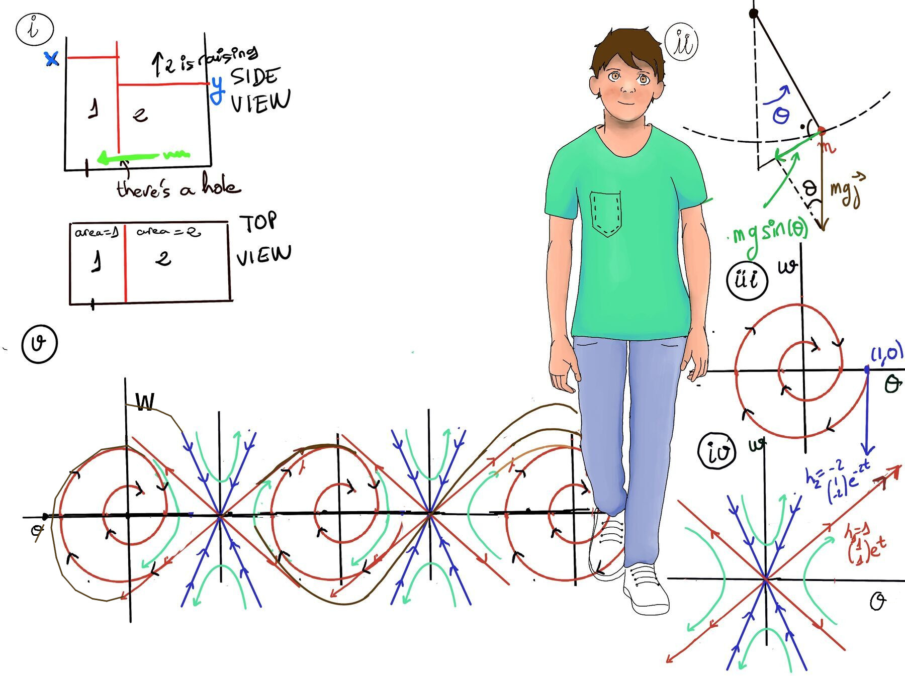
Consider a lightly damped pendulum, which consists of a mass m attached to a rod of length l swinging back and force under the influence of gravity and a damping force. The angle $\theta$ between the rod and the vertical axis describes the pendulum’s position (Refer to Figure ii for a visual representation and aid in understanding it).

Deriving the Equations of Motion

The dynamics of the pendulum’s motion are governed by Newton’s Second Law, which states that the net force acting on the pendulum in the tangential direction is equal to the mass times the angular acceleration, $m\vec{a} = \vec{F}$. Since linear acceleration $a$ along the circular path is related to angular acceleration $\theta''$ by $a = l\theta''$, we have: $m l \theta'' = \vec{F}$

The forces acting on the pendulum are:

1. The force of gravity. This acts in the direction of the center of the Earth (downwards), and its tangential component is given by $-mg\sin(\theta)$ where g is the acceleration due to gravity. The negative sign indicates that gravity acts as a restoring force, pulling the pendulum back to the equilibrium position ($\theta = 0$).
2. The damping force. This opposes the velocity of the pendulum. It is proportional to the angular velocity $\theta'$, represented by $-c_1 l \theta'$, where $c_1$ is the damping coefficient (units of $\text{kg} \cdot \text{m}^2/\text{s}$).

Thus, Newton’s equation be $m l \theta'' = -mg\sin(\theta) - c_1 l \theta'$

By dividing everything by $m l$, we simplify this to: $\theta'' + \frac{c_1}{m}\theta' + \frac{g}{l}\sin(\theta) = 0$

To make the notation more compact, we define constants $c = \frac{c_1}{m}$ (the damping ratio) and $k = \frac{g}{l}$ (related to the natural frequency of the pendulum). This yields the non-linear second-order differential equation: $\theta'' + c\theta' + k\sin(\theta) = 0$

It is non-linear specifically due to the $\sin(\theta)$ term.

Converting to a First-Order System

To analyze this system, we convert it into a first-order system by introducing a new variable $w = \theta'$ (the angular velocity).

Differentiating our new variable gives $w' = \theta''$. Substituting this into our simplified Newton’s equation gives: $w' = -k\sin(\theta) - c\theta' = -k\sin(\theta) - cw$

This leads to the following system of equations:

$$\begin{cases} \theta' = w \\ w' = -k\sin(\theta) - cw \end{cases}$$

This is now a system of two first-order equations in the variables $\theta$ and $w$.

For this example, we will examine a specific under-damped (lightly damped) case, where $c = 1$ and $k = 2$. The system becomes:

$$\begin{cases} \theta' = w \\ w' = -2\sin(\theta) - w \end{cases}$$

Step 1: Find Critical Points

Critical points (equilibrium points) are points where both derivatives are zero, i.e., where the system is in equilibrium (in a state of rest). Setting the right-hand sides of both equations to zero:

$\begin{cases} f(x, y) = 0 \\\ g(x, y) = 0 \end{cases}$

In our example, we need to solve:

$\begin{cases} w = 0 \\\ -2\sin(\theta) - w = 0 \end{cases}$

Substituting $w = 0$ into the second equation yields: $-2\sin(\theta) = 0 \implies \sin(\theta) = 0$

The solutions for this are $\theta = n\pi$, where $n \in \mathbb{Z}$. Thus, the critical points are $(\theta, w) = (n\pi, 0)$. These correspond to the pendulum being perfectly at rest ($\theta' = 0$) at various angles: $0, \pm\pi, \pm2\pi, \dots$

Physically, there are two notable types of critical points:

• $(\theta, w) = (0, 0)$ (and even multiples of $\pi$): Corresponding to a stable equilibrium. The pendulum is hanging straight down and at rest.
• $(\theta, w) = (\pi, 0)$ (and odd multiples of $\pi$): Corresponding to an unstable equilibrium. The pendulum is perfectly balanced in the inverted position.

Step 2: Linearizing the System Near the Critical Points

To analyze the behavior near each critical point, we linearize the system. This could involve approximating the non-linear functions with linear ones by taking their Taylor expansion around the critical point. Near $\theta = 0$, we can use the approximation $\sin(\theta) \approx \theta$. The system then becomes:

$\begin{cases} \theta' = w \\\ w' = -2\theta -w\end{cases}$

This is a linear system and can be written in matrix form as:

$(\begin{smallmatrix}\theta'\\\ w'\end{smallmatrix}) = (\begin{smallmatrix}0 & 1\\\ -2 & -1\end{smallmatrix})(\begin{smallmatrix}\theta\\\ w\end{smallmatrix})$

To determine the behavior of the system, we calculate the eigenvalues of the matrix. The characteristic equation is:

$det(\begin{smallmatrix}0-λ & 1\\\ -2 & -1-λ\end{smallmatrix}) = (−λ)(−1−λ)−(−2)(1)=λ(λ+1)−(−2)= λ^2 + λ +2 = 0 ↭ λ = \frac{-1±\sqrt{1-8}}{2} = \frac{-1±\sqrt{-7}}{2}=\frac{-1±i\sqrt{7}}{2}$.

The eigenvalues are complex with a negative real part indicating a spiral sink.

• The negative real part ($\frac{-1}{2}$) indicates exponential decay, meaning that trajectories spiral (or shrink) inward toward the critical point as time progresses.
• The imaginary part ($\frac{\sqrt{7}}{2}$) causes the oscillatory (spiraling) behavior.

Thus, near $(\theta, w)= (0, 0)$, the system exhibits a stable spiral or spiral sink. Trajectories spiral inward in a clockwise or counterclockwise fashion, depending on initial conditions, representing damped oscillations of the pendulum returning gradually to the equilibrium position (to rest at the bottom).

The motion of the pendulum will involve spirals that gradually shrink in size, representing the damping effect. The negative real part leads to the shrinking (loss of energy), while the oscillations correspond to the spiraling (swinging back and forth) until it returns to rest at the bottom.

Consider $(\theta, w) = (1, 0)$, $(\begin{smallmatrix}\theta'\\\ w'\end{smallmatrix}) = (\begin{smallmatrix}0 & 1\\\ -2 & -1\end{smallmatrix})(\begin{smallmatrix}\theta\\\ w\end{smallmatrix}) = (\begin{smallmatrix}0 & 1\\\ -2 & -1\end{smallmatrix})(\begin{smallmatrix}1\\\ 0\end{smallmatrix}) = (\begin{smallmatrix}0\\\ -2\end{smallmatrix})$

This show that the velocity is pulling downwards, so the motion is clockwise. Near (0, 0), the system exhibits spiral sinks, with trajectories spiraling inward in a clockwise direction. (Refer to Figure iii for a visual representation and aid in understanding it)

Behavior Around $(\pi, 0)$. At $(\pi, 0)$ we cannot approximate $\sin(\theta)$ as $\theta$. We compute the Jacobian matrix, which effectively linearizes the system by taking the multivariable Taylor expansion around the critical points.:

For a system:

$\begin{cases} \theta^′ = f(\theta, w) \\\ w^′ = g(\theta, w) \end{cases}$

The Jacobian matrix at a critical point $(\theta_0, w_0)$ is:

$J(\theta, w) = (\begin{matrix}\frac{\partial f}{\partial \theta} & \frac{\partial f}{\partial w}\\\ \frac{\partial g}{\partial \theta} & \frac{\partial g}{\partial w}\end{matrix})\bigg|_{\theta_0, w_0} = (\begin{matrix}f_\theta & f_w\\\ g_\theta & g_w\end{matrix})\bigg|_{\theta_0, w_0}$, and this is the matrix of the linearized system.

$(\begin{matrix}\frac{∂w}{∂θ} & \frac{∂w}{∂w}\\\ \frac{∂(-2sin(θ)-w)}{∂θ} & \frac{∂(-2sin(θ)-w)}{∂w}\end{matrix}) = (\begin{matrix}0 & 1\\\ -2cos(θ) & -1\end{matrix})$

Evaluate at (0, 0): $J_{(0, 0)} = (\begin{matrix}0 & 1\\\ -2 & -1\end{matrix})$. This is consistent with the previous result.

Evaluating the Jacobian at the inverted position gives: $(\pi, 0)$: $J(\pi, 0) = \begin{pmatrix} 0 & 1 \\ -2\cos(\pi) & -1 \end{pmatrix} = \begin{pmatrix} 0 & 1 \\ 2 & -1 \end{pmatrix}$

Finding the eigenvalues: $\det \begin{pmatrix} -\lambda & 1 \\ 2 & -1-\lambda \end{pmatrix} = (-\lambda)(-1-\lambda) - (2)(1) = \lambda^2 + \lambda - 2 = 0$

Factoring yields $(\lambda + 2)(\lambda - 1) = 0$, giving eigenvalues $\lambda_1 = 1$ and $\lambda_2 = -2$.

Having real eigenvalues with opposite signs strictly indicates a saddle point.

$\lambda = 1, (J-\lambda I)\vec{v} = \vec{0} ↭ (\begin{smallmatrix}-1 & 1\\\ 2 & -2\end{smallmatrix})(\begin{smallmatrix}a_1\\\ a_2\end{smallmatrix}) = \vec{0}$

$\begin{cases} -a_1 + a_2 = 0 \\\ 2a_1 -2a_2 = 0 \end{cases}$

$-a_1 + a_2 = 0 \implies a_1 = a_2 =[\text{Simplicity}] 1$. The second equation is redundant. Eigenvector: $(\begin{smallmatrix}1\\\ 1\end{smallmatrix})$. The solution is $(\begin{smallmatrix}1\\\ 1\end{smallmatrix})e^{t}$

$\lambda = -2, (J-\lambda I)\vec{v} = \vec{0} ↭ (\begin{smallmatrix}2 & 1\\\ 2 & 1\end{smallmatrix})(\begin{smallmatrix}a_1\\\ a_2\end{smallmatrix}) = \vec{0}$

$\begin{cases} 2a_1 + a_2 = 0 \\\ 2a_1 + a_2 = 0 \end{cases}$

$2a_1 + a_2 = 0 \implies a_2 = -2a_1$. Eigenvector: $(\begin{smallmatrix}1\\\ -2\end{smallmatrix})$. The solution is $(\begin{smallmatrix}1\\\ -2\end{smallmatrix})e^{-2t}$

The eigenvalues are real and have opposite signs. This indicates a saddle point at $(\pi, 0)$. The general solution is $\boxed{c_1(\begin{smallmatrix}1\\\ 1\end{smallmatrix})e^{t}+c_2(\begin{smallmatrix}1\\\ -2\end{smallmatrix})e^{-2t}}$

• It represents the pendulum inverted at the top $(\theta = \pi)$.
• Unstable Manifold. The positive eigenvalue $\lambda = 1$ corresponds to an unstable direction $\vec{v_1}=(\begin{smallmatrix}1\\\ 1\end{smallmatrix})$. Trajectories along this line $w = \theta$ move away from the critical point $(\pi, 0)$. $c_2 = 0, c_1 = 1, \vec{v_1}=(\begin{smallmatrix}1\\\ 1\end{smallmatrix}), y = x$.
• Stable Manifold. The negative eigenvalue $\lambda = -2$ corresponds to a stable direction $\vec{v_2}=(\begin{smallmatrix}1\\\ -2\end{smallmatrix})$ (trajectories along this line $w = -2\theta$ move toward the critical point $(\pi, 0)$). $c_1 = 0, c_2 = 1, \vec{v_2}=(\begin{smallmatrix}1\\\ -2\end{smallmatrix}), y = -2x$.
• Trajectories approach the critical point along one direction and diverge along another. Physically, the inverted pendulum position is unstable; any slight perturbation causes it to fall away from $\theta = \pi$. A perfect initial push (the stable manifold) might theoretically balance it, but practically it will deviate along the unstable manifold.

Near $(\pi, 0)$, the system exhibits a saddle point, with trajectories diverging in one direction and converging in another (Refer to Figure iv for a visual representation and aid in understanding it).

Step 3. Plot trajectories around each critical point and then add some more. (Refer to Figure v for a visual representation and aid in understanding it)

The global behavior demonstrates the periodic nature of the pendulum system (since $\sin(\theta)$ is periodic with period $2\pi$), with repeated critical points at multiples of $\theta, \theta = n\pi$ alternating between stable spirals (damped oscillations) and saddle points (more complex behavior).

Bibliography

1. NPTEL-NOC IITM, Introduction to Galois Theory.
2. Algebra, Second Edition, by Michael Artin.
3. LibreTexts, Calculus and Calculus 3e (Apex). Abstract and Geometric Algebra, Abstract Algebra: Theory and Applications (Judson).
4. Field and Galois Theory, by Patrick Morandi. Springer.
5. Michael Penn, and MathMajor.
6. Contemporary Abstract Algebra, Joseph, A. Gallian.
7. YouTube’s Andrew Misseldine: Calculus. College Algebra and Abstract Algebra.
8. MIT OpenCourseWare [18.03 Differential Equations, Spring 2006], YouTube by MIT OpenCourseWare.
9. Calculus Early Transcendentals: Differential & Multi-Variable Calculus for Social Sciences.