Radioactive Decay Chains and Modeling

We shall fight on the beaches, we shall fight on the landing grounds, we shall fight in the fields and in the streets, we shall fight in the hills; we shall never surrender, Winston Churchill

Recall

Definition. A differential equation is an equation that involves one or more dependent variables, their derivatives with respect to one or more independent variables, and the independent variables themselves, e.g., $\frac{dy}{dx} = 3x +5y, y' + y = 4xcos(2x), \frac{dy}{dx} = x^2y+y, etc.$

It involves (e.g., $\frac{dy}{dx} = 3x +5y$):

• Dependent variables: Variables that depend on one or more other variables (y).
• Independent variables: Variables upon which the dependent variables depend (x).
• Derivatives: Rates at which the dependent variables change with respect to the independent variables, $\frac{dy}{dx}$

Basic linear ODE

In mathematics, a linear ordinary differential equation (ODE) is an equation involving an unknown function and its derivatives, characterized by the property that both the function and its derivatives appear linearly. This means that the unknown function and its derivatives are raised only to the first power. They are never multiplied together, nor are they composed within nonlinear functions (such as $\sin(y)$ or $e^y$). The general form for a first-order linear ODE is: a(x)y’ + b(x)y = c(x).

This property of linearity is fundamental. While most physical systems are inherently nonlinear, many can be accurately approximated by linear models over a specific range. This linearity allows mathematicians and engineers to utilize a vast and powerful toolkit of analytical solution methods that are unavailable for nonlinear systems. Consequently, linear ODEs are the bedrock of modeling in numerous fields, including:

• Fluid Dynamics: Describing fluid flow conditions under simplifications where the governing equations can be linearized.
• Electrical Circuits: Analyzing the behavior of circuits containing linear components like resistors, capacitors, and inductors (RLC circuits).
• Mechanical Vibrations: Modeling the motion of oscillating systems, such as springs and pendulums, in regimes where Hooke’s law —a linear relationship— holds.
• Radioactive Decay: Describing the constant proportional rate at which unstable atomic nuclei lose energy, resulting in exponential decay.

In this article, we will explore different forms of linear ODEs, their applications, and their solutions, with a focus on understanding their behavior in real-world contexts.

Mathematical Definition of Linearity

An ODE of order n is linear if it can be expressed in the form: $a_n(t)\frac{d^ny}{dt^n} +a_{n-1}(t)\frac{d^{n-1}y}{dt^{n-1}} + ··· + a_1(t)\frac{dy}{dt} + a_0(t)y = q(t)$ where

• y(t) is the unknown function (dependent variable).
• i is the independent variable.
• $\frac{d^ky}{dt^k}$ are the derivatives of y with respect to t.
• a_i(t) are known coefficient functions of t. They can be constants or functions of t, but they do not depend on y.
• q(t) is a known function, often called the forcing function or input.

The function y and its derivatives appear to the first power and are not multiplied together.

Radioactive Decay Chains and Modeling

Radioactive decay is a natural, stochastic process by which an unstable atomic nucleus loses energy by emitting radiation. This phenomenon can be precisely modeled on the macroscopic scale using first-order linear ordinary differential equations (ODEs). In this context, we will explore a decay chain system: one radioactive substance A decays into another radioactive substance B, which subsequently decays into a stable end product C.

Consider the specific parameters of this chain (A→B→C):

• Substance A: A decays into substance B at a rate proportional to the current amount of A, A(t). Let $k_1$ be the decay constant for substance A.

• Substance B: It accumulates due to the decay of A and simultaneously undergoes its own decay into substance C. B decays at a rate proportional to the amount of B, too. Let $k_2$ be the decay constant for substance B.

Modeling the Dynamics of Substances A and B

Modeling Substance A

The rate at which substance A decays is proportional to its current amount. This relationship is expressed by the homogeneous, separable differential equation:

$$\frac{dA}{dt} = -k_1A$$

.

We can solve this using standard Separation of variables:

$\frac{dA}{A} = -k_1dt ↭[\text{Integrate both sides}] \int \frac{dA}{A} = \int -k_1dt ↭ ln|A| = -k_1t + C_1$

Solving for A(t) yields the classic exponential decay model: $A(t) = e^{-k_1t+C_1} = A_0e^{-k_1t}$ where $A_0 = e^{C_1}$ is the initial amount of substance A at t = 0.

The amount of substance A decreases exponentially over time.

Modeling Substance B

Substance B is subject to two competing rates: production (gain) and decay (loss).

1. Rate of Production: Since substance A decays into B, the production rate of B is equal to the rate A is decreasing: $\frac{-dA}{dt} = k_1A(t)$

2. Rate of Decay: Substance B decays at a rate proportional to its own amount: $\frac{dB}{dt} = -k_2B(t)$

The rate of change of B(t) is the net difference between production and decay: $\frac{dB}{dt} = \text{Production - Decay} = k_1A(t) -k_2B(t)$

Substituting the known expression for A(t), $A(t) = A_0e^{-k_1t}$, into the equation yields a first-order, non-homogeneous linear ODE in standard form:

$$\frac{dB}{dt} = k_1A_0e^{-k_1t}-k_2B(t) \implies \frac{dB}{dt} + \boxed{k_2B(t) = k_1A_0e^{-k_1t}}$$

.

This is a first-order linear ODE of the form y' + P(t)y = Q(t). The solution describes the amount of B as it accumulates and decays over time,

Solving the Differential Equation for B(t)

1. Find the Integrating Factor: $μ(t) = e^{\int P(t)dt}= e^{\int k_2dt} = e^{k_2·t}$
2. Multiply Both Sides by μ(t): $e^{k_2·t}\frac{dB}{dt}+ e^{k_2·t}k_2B = k_1A_0e^{-k_1t}e^{k_2·t}↭[Simplify] \frac{d}{dt}(e^{k_2·t}B(t)) = k_1A_0e^{(k_2-k_1)t}$
3. Integrate Both Sides: $\int \frac{d}{dt}(e^{k_2·t}B(t)) = \int k_1A_0e^{(k_2-k_1)t} ↭ e^{k_2·t}B(t) = \int k_1A_0e^{(k_2-k_1)t} + C$ where C is the constant of integration.
4. Evaluate the Integral: The result of this integration depends entirely on whether $k_1$ equals $k_2$. This is a crucial physical distinction. ($\star$) Case 1. Standard Case: $k_1 \ne k_2$, $e^{k_2·t}B(t) = \frac{k_1A_0}{k_2-k_1}e^{(k_2-k_1)t} + C$.
   ($\star$) Case 2: $k_1 = k_2 = k$, $e^{k_2·t}B(t) = k_1A_0t + C$
5. Determining the General Solution for B(t). Now, we solve for B(t) in both distinct cases.

($\star$) Case 1. Standard Case: $k_1 \ne k_2$, $B(t) = e^{-k_2·t}(\frac{k_1A_0}{k_2-k_1}e^{(k_2-k_1)t} + C) \implies \boxed{B(t) = \frac{k_1A_0}{k_2-k_1}e^{-k_1t} + Ce^{-k_2·t}}$

Initial Conditions: Assume that at $t = 0$, an initial amount $B(0) = B_0$ is present.

$B_0 = \frac{k_1A_0}{k_2-k_1}e^{0} + Ce^{0} \implies B_0 = \frac{k_1A_0}{k_2-k_1} + C \implies C = B_0 - \frac{k_1A_0}{k_2-k_1}$

$\mathbf{B(t) = \frac{k_1A_0}{k_2-k_1}e^{-k_1t} + \left(B_0 - \frac{k_1A_0}{k_2-k_1}\right)e^{-k_2t}}$

Note: In typical natural scenarios where a parent substance A is introduced to a new environment, we can assume B(0) = 0. The expression simplifies to: $\boxed{B(t) = \frac{k_1A_0}{k_2-k_1}(e^{-k_1t} - e^{-k_2t})}$

($\star$) Case 2: $k_1 = k_2 = k$, $\boxed{B(t) = e^{-k·t}(kA_0t + C)}$

Initial Conditions: Assume $B(0) = B_0$.

Then, $B_0 = e^{0}(kA_0\cdot 0 + C) \implies B_0 = C$

Therefore, $\mathbf{B(t) = e^{-kt}(kA_0t + B_0)} = (B_0 + kA_0t)e^{-kt}$

Physical Interpretation

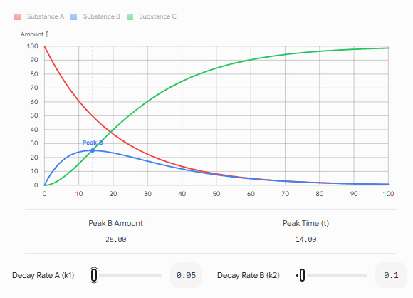
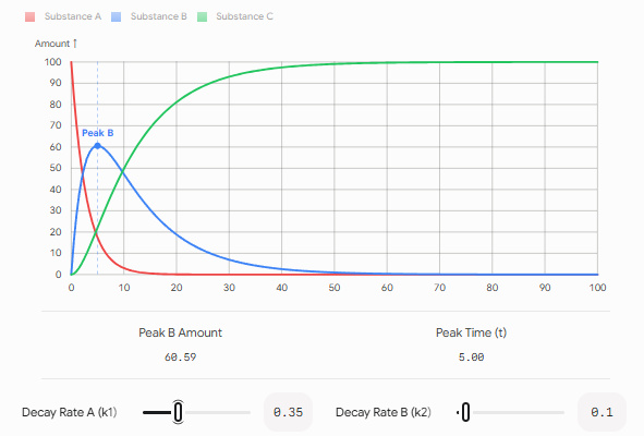
• Initial Growth and Peak for B. Initially, $B(t)$ must increase. If $B_0=0$, the rate of production ($k_1A$) is positive and maximum at $t=0$, while the rate of decay ($-k_2B$) is zero. $B(t)$ will rise, reach a maximum peak (the point where Production equals Decay: $k_1A(t_{\text{peak}}) = k_2B(t_{\text{peak}})$), and then inevitably decline as $A(t)$ is depleted.

• Regime: Transient Equilibrium ($k_1 < k_2$): Substance $A$ decays slowly, and $B$ decays relatively quickly. The intermediate product $B(t)$ cannot accumulate substantially. Its curve will peak quickly and then track the slow, steady decay of its parent, $A$.

• Regime: “Secular” or Strong Accumulation ($k_1 > k_2$): Substance $A$ decays rapidly into $B$, while $B$ decays much slower. This causes $B$ to accumulate strongly, reaching a high peak that lingers before its much slower natural decay constant dominates the dynamics. This form approaches standard decay of $B$ after $A$ is effectively extinguished.

Special Case Sidebar: The Growing System, $\frac{dy}{dt}-ay = q(t)$

A differential equation with a structure similar to the standard non-homogeneous linear form, but with a positive coefficient for $y$ in the general form $y' - ay = q(t)$, leads to completely different physical behavior—exponential growth. This form is used to model systems that expand without bound, such as population growth in a resource-rich environment or neutron multiplication within a nuclear reactor core.

1. It is already in standard form: $\frac{dy}{dt}-ay = q(t)$ where a > 0 is the growth constant and q(t) is a continuous source or input function. To solve it, we use the integrating factor method.
2. Find the Integrating Factor: $μ(t) = e^{\int -adt} = e^{-at}$
3. Multiply Both Sides by μ(t): $e^{-at}\frac{dy}{dt}-ae^{-at}y = e^{-at}q(t) ↭ \frac{d}{dt}(e^{-at}y) = e^{-at}q(t)$
4. Integrate Both Sides: $\int \frac{d}{dt}(e^{-at}y)dt = \int e^{-at}q(t)dt ↭ e^{-at}y = \int e^{-at}q(t)dt + C$
5. Solve for y: $\boxed{y(t) = e^{at}\int q(t)e^{-at}dt + ce^{at}}$.

Identification of Behavior

The behavior depends crucially on the growth parameter $a > 0$. Unlike the earlier natural transient terms ($Ce^{-k_2t}$) which decayed to zero, the term $y_h(t)=Ce^{at}$ is no longer transient, but grows exponentially since $a > 0$.

This system is inherently unstable. If $C \neq 0$ (meaning the system was not in a perfect, albeit unstable, mathematical equilibrium at $t=0$), the homogeneous solution grows without bound. The particular solution depends on q(t) and may counteract or reinforce the exponential growth.

The constant $C$ is strictly determined by the initial condition $y(t_0) = y_0$. Small, almost imperceptible differences in the starting condition $y_0$ can lead to massive differences in $y(t)$ as time increases due to the exponential growth.

Example with Constant Source Term q(t) = q₀

This is a very common scenario for modeling a system with growth and a constant, external supply (e.g., constant resource flow in population dynamics).

The equation becomes: $\frac{dy}{dt}-ay = q_0$.

1. Integrate: $\int q(t)e^{-at}dt = \int q_0e^{-at}dt = -\frac{q_0}{a}e^{-at} + C'$ (Since C’ will be absorbed into C, we can omit it).
2. Simplify General Solution: $y(t) = e^{at}(-\frac{q_0}{a}e^{-at} + C) = -\frac{q_0}{a} + Ce^{at}$
3. Apply initial condition. If y(0) = y₀, $y_0 = -\frac{q_0}{a} + Ce^{a·0} = -\frac{q_0}{a} + C [\text{Solve for C}] C = y_0 + \frac{q_0}{a}$.
4. Final explicit solution: $\boxed{y(t) = -\frac{q_0}{a} + (y_0 + \frac{q_0}{a})e^{at}}$

This solution highlights the critical role of the initial condition. Define $C = y_0 + \frac{q_0}{a}e^{at}$. Then, $y(t) = -\frac{q_0}{a} + C e^{at}$

The steady-state solution (equilibrium) is only $-\frac{q_0}{a}$ when a < 0. The equilibrium is stable; all solutions converge to $y_0$. For growth (a > 0), this is an unstable equilibrium point. The term $C e^{at}$ is the transient, determined entirely by the initial condition.

If the initial condition is perfectly set such that $y_0 = -\frac{q_0}{a}$, the constant $C=0$ and the growth term vanishes; $y(t)$ remains constant forever, $y(t) = -\frac{q_0}{a}$.

In any other scenario ($y_0 \neq -\frac{q_0}{a}$), the growth constant $C$ is non-zero, and the solution is dominated by the exponential term, diverging rapidly. As $t \to \infty$, the exponential term dominates, $\lim_{t \to ∞} y(t) = \text{sign}\left(y_0 + \frac{q_0}{a}\right) \cdot \infty$

Bibliography

1. NPTEL-NOC IITM, Introduction to Galois Theory.
2. Algebra, Second Edition, by Michael Artin.
3. LibreTexts, Calculus and Calculus 3e (Apex). Abstract and Geometric Algebra, Abstract Algebra: Theory and Applications (Judson).
4. Field and Galois Theory, by Patrick Morandi. Springer.
5. Michael Penn, and MathMajor.
6. Contemporary Abstract Algebra, Joseph, A. Gallian.
7. YouTube’s Andrew Misseldine: Calculus. College Algebra and Abstract Algebra.
8. MIT OpenCourseWare [18.03 Differential Equations, Spring 2006], YouTube by MIT OpenCourseWare.
9. Calculus Early Transcendentals: Differential & Multi-Variable Calculus for Social Sciences.