Limit Cycles in Non-Linear Autonomous Systems

If you’re going through hell, keep on going, Winston Churchill.

Limit Cycles in Non-Linear Autonomous System

In the study of differential equations and dynamical systems, non-linear autonomous systems are of great interest because they model complex, real-world phenomena that linear systems simply cannot—such as the beating of a heart, predator-prey oscillations, and electronic oscillator circuits. One of the most fascinating and exclusively non-linear phenomena exhibited by such systems is the occurrence of limit cycles.

We consider a general two-dimensional non-linear autonomous system of the form:

$\begin{cases} x' = f(x, y) \\\ y' = g(x, y) \end{cases}$ where:

• x’ and y’ denote the time derivatives $\frac{dx}{dt}$ and $\frac{dy}{dt}$, respectively.
• f(x, y) and g(x, y) are non-linear functions that govern the time evolution of the variables x and y. This system describes how the state (x, y) evolves over time, based on their current values.

By “autonomous,” we mean that these functions do not explicitly depend on time. The evolution of the system depends only on the current state (x, y), not on what time it is.

Visualizing the System: The Velocity Field

To gain a better, intuitive understanding of the behavior of the system's behavior, we can represent it as a velocity (or vector) field $\vec{F}$ in the phase plane. The velocity field is defined as: $\boxed{\vec{F} = f(x, y)\hat{\mathbf{i}}+g(x, y)\hat{\mathbf{j}}}$ where

• $f(x, y)\hat{\mathbf{i}}$ represents the velocity component in the x-direction.
• $g(x, y)\hat{\mathbf{j}}$ represents the velocity component in the y-direction.
• $\hat{\mathbf{i}}$ and $\hat{\mathbf{j}}$ are standard unit vectors in the x and y axes, respectively.

This vector field describes how the values of x and y change over time at every single point in the plane. If we think of $(x(t), y(t))$ as the position of a “particle” moving in the plane, $\vec{F}(x, y)$ tells us the exact instantaneous direction and speed of that particle.

Trajectories in the Phase Plane

Solutions to the system are pairs of functions x(t) and y(t), but geometrically, they are trajectories or paths traced out by the evolving system in the xy-plane (phase plane).

These trajectories follow the direction of the vector field $\vec{F}$, meaning that at any point along the trajectory, the tangent vector to the path is precisely $\vec{F}(x, y)$.

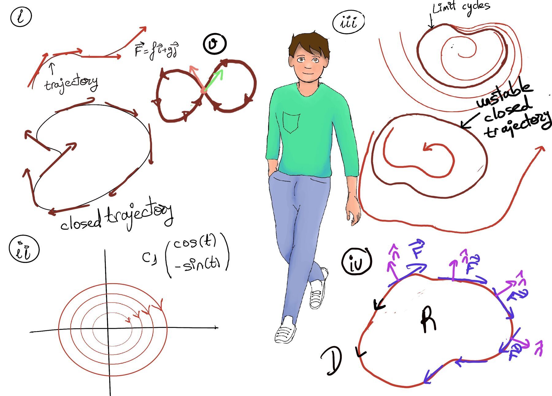
Refer to Figure i for a visual representation and aid in understanding it. Different initial conditions may lead to different trajectories, but these trajectories can never cross each other. This is a consequence of the uniqueness theorem for differential equations: if two distinct solutions crossed at a point, that specific point would have two different future evolutions (two different arrows pointing in different directions), which is impossible in a deterministic autonomous system.

Critical Points and Local Stability

A critical point (or equilibrium point) of the system occurs where the velocity field vanishes —i.e., where the system's rate of change is zero. Mathematically, this happens when $f(x_0, y_0) = 0 \quad \text{and} \quad g(x_0, y_0) = 0$, meaning that the velocity at the point $(x_0, y_0)$ is zero. At such points, the system is at perfect equilibrium, that is, there is no motion, and the solution remains constant over time indefinitely.

In terms of the field, these points are where: $\vec{F}(x_0, y_0) = f(x_0, y_0)\hat{\mathbf{i}}+g(x_0, y_0)\hat{\mathbf{j}} = \vec{0}$

Critical points are important because they often represent stable or unstable equilibrium states where the system tends to “settle” or from which it may “escape” in the long term, depending on the nature of the equilibrium.

The local behavior near critical points is analyzed using linearization via the Jacobian matrix: $J = \begin{pmatrix} \frac{\partial f}{\partial x} & \frac{\partial f}{\partial y} \\ \frac{\partial g}{\partial x} & \frac{\partial g}{\partial y} \end{pmatrix}\Bigg|_{(x_0, y_0)}$

The eigenvalues of J determine the local behavior near the critical point:

• Stable Node/Focus. If both eigenvalues have negative real parts, the critical point is a stable node or stable focus. Solutions or trajectories near this critical point converge to it as $t \to \infty$.
• Unstable Node/Focus. If both eigenvalues have positive real parts, it’s an unstable node or unstable focus. Solutions or trajectories near this critical point diverge or move away from it as $t \to \infty$.
• Saddle Point. If eigenvalues are real and of opposite signs, the critical point is a saddle point. Solutions approach the critical point along one eigenvector and move away along the other, making it unstable.
• Center. If eigenvalues are purely imaginary conjugates (with zero real part), nearby solutions or trajectories circle around the equilibrium. The critical point is a center. Solutions orbit around the critical point without converging or diverging.

  Trajectories (center) form continuous, nested, closed loops around the equilibrium (like planets orbiting a star).

Closed Trajectories vs. Limit Cycles

A closed trajectory is a path in the xy-plane that loops back onto itself (to its starting point) and then repeats indefinitely. In other words, if a trajectory is closed, the system exhibits periodic behavior, that is, after a certain period T, the system returns exactly to its initial state, and this cycle repeats over and over.

Geometrically, a closed trajectory represents a periodic solution (x(t), y(t)) such that: x(t + T) = x(t), y(t + T) = y(t) for all t.

Importantly, a closed trajectory does not cross itself —the system cannot have two different velocity directions at the same point due to the uniqueness of solutions in differential equations (Refer to Figure v for a visual representation and aid in understanding it). This property ensures that the system’s motion is uniquely determined by the initial conditions and evolves in a smooth, continuous manner.

In linear systems, closed trajectories are “centers.” They exist as infinite, nested rings. If you bump a linear system, it simply shifts to a slightly larger or smaller nested ring and stays there.

Example: A Simple Harmonic Oscillator

The simple harmonic oscillator is a fundamental example in differential equations, classical mechanics, and physics, representing systems that exhibit purely periodic motion, such as springs and pendulums under ideal conditions.

Common real-world examples include a mass attached to an undamped or frictionless spring (obeying Hooke’s law) or a small-angle pendulum, each oscillating around a stable equilibrium position. The simple harmonic oscillator is linear, conservative (there is no energy loss to damping or friction), and its solutions are sinusoidal, indicating perfect, perpetual periodic motion.

Consider the system of differential equations: $\begin{cases} x' = y \\\ y' = -x \end{cases}$ where x = x(t) and y = y(t) are functions of time t (two variables that oscillate over time), and x’ and y’ denote derivatives of x and y, respectively with respect to time. This system describes how the variables x and y evolve over time, with the rate of change of each variable depending directly on the other.

By differentiating the first equation and substituting the second, we can derive a second-order differential equation for $x$ alone: $x'' = y' = -x \implies x'' + x = 0$ which is the classic equation of a simple harmonic oscillator. In other words, this system describes a simple harmonic oscillator.

The matrix representation of the system is: $\vec{x'} = Ax$ where A = $(\begin{smallmatrix}0 & 1\\\ -1 & 0\end{smallmatrix})$ is the coefficient matrix, and $\vec{x} = (\begin{smallmatrix}x\\\ y\end{smallmatrix})$ is the state vector. This compact form allows us to use linear algebra techniques to solve the system.

Finding Eigenvalues and Eigenvectors

To find the eigenvalues, we solve the characteristic equation: $\det(A-\lambda I) = 0$: $\det\begin{pmatrix} -\lambda & 1 \\ -1 & -\lambda \end{pmatrix} = (-\lambda)(-\lambda) - (1)(-1) = \lambda^2 + 1 = 0 \implies \lambda^2 = -1$. The eigenvalues are $\lambda_1 = i$ and $\lambda_2 = -i$.

The eigenvalues are purely imaginary. This indicates that the system exhibits purely rotational (oscillatory) behavior in the xy-plane (phase plane). Trajectories in the (x, y)-plane will rotate continuously around the origin, neither spiraling inward nor outward.

To find the eigenvectors, we substitute each eigenvalue back into $(A-\lambda I)\vec{v} = \vec{0}$.

For $\lambda_1 = i$: $(\begin{smallmatrix}-i & 1\\\ -1 & -i\end{smallmatrix})(\begin{smallmatrix}a_1\\\ a_2\end{smallmatrix}) = (\begin{smallmatrix}0\\\ 0\end{smallmatrix})$

From the first equation: $-ia_1 +a_2 = 0 \implies a_2 = ia_1$. From the second row: $-a_1 -ia_2 = 0$ ⇒[Substitute $a_2 = ia_1$] $-a_1 -i(ia_1) = -a_1 + a_1 = 0$. We can choose $a_1 = 1$ (since eigenvectors are determined up to a scalar multiple). Therefore, the eigenvector is: $\vec{v_1}=(\begin{smallmatrix}1\\\ i\end{smallmatrix})$

For $\lambda_2 = -i$, $(\begin{smallmatrix}i & 1\\\ -1 & i\end{smallmatrix})(\begin{smallmatrix}a_1\\\ a_2\end{smallmatrix}) = (\begin{smallmatrix}0\\\ 0\end{smallmatrix})$

From the first equation: $ia_1 +a_2 = 0 \implies a_2 = -ia_1$. Choosing $a_1 = 1$, we have: $\vec{v_2}=(\begin{smallmatrix}1\\\ -i\end{smallmatrix})$

Constructing the Real Solution

The general complex solution to the system is a linear combination of the eigenvectors multiplied by their exponential eigenvalues: $\boxed{\vec{x}(t) = c_1e^{it}\vec{v_1} + c_2e^{-it}\vec{v_2}}$ where $c_1$ and $c_2$ are complex constants determined by initial conditions.

Substituting the eigenvectors: $\vec{x}(t) = c_1e^{it}(\begin{smallmatrix}1\\\ i\end{smallmatrix})+c_2e^{-it}(\begin{smallmatrix}1\\\ -i\end{smallmatrix})$

To find real-valued solutions, we express the complex exponentials using Euler’s formula: $e^{it} = cos(t) + isin(t), e^{-it} = cos(t) - isin(t)$ and extract the real and imaginary part of $e^{-it}\vec{v_1}$

$e^{it}\vec{v_1} = (\cos t + i\sin t)\begin{pmatrix} 1 \\ i \end{pmatrix} = \begin{pmatrix} \cos t + i\sin t \\ i\cos t - \sin t \end{pmatrix} = \begin{pmatrix} \cos t \\ -\sin t \end{pmatrix} + i\begin{pmatrix} \sin t \\ \cos t \end{pmatrix}$

• First Real Solution. Take the real part of $e^{it}\vec{v_1}$: $\mathbb{R}[e^{it}\vec{v_1}] = (\begin{smallmatrix}cos(t)\\\ -sin(t)\end{smallmatrix})$

• Second Real Solution. Take the imaginary part of $e^{it}\vec{v_1}$: $\mathbb{ℑ}[e^{it}\vec{v_1}] = (\begin{smallmatrix}sin(t)\\\ cos(t)\end{smallmatrix})$

Therefore, the general real solution is: $\boxed{c_1(\begin{smallmatrix}cos(t)\\\ -sin(t)\end{smallmatrix})+c_2(\begin{smallmatrix}sin(t)\\\ cos(t)\end{smallmatrix})}$ where $c_1$ and $c_2$ are real constants determined by initial conditions.

The solutions x(t) and y(t) represent sinusoidal functions with the same frequency but possibly different amplitudes and phases.

Circular Trajectories (Centers)

For the simple harmonic oscillator, the trajectories in the phase plane form a family of concentric circles centered at the origin, representing periodic motion Each trajectory is a closed curve, and the motion goes around clockwise indefinitely, which is typical of simple harmonic oscillators. Refer to Figure ii for a visual representation and aid in understanding it.

For the simple harmonic oscillator, the trajectories are circles centered at the origin. To see this, consider the expressions $x(t) = c_1\cos(t) + c_2\sin(t), y(t) = -c_1\sin(t) + c_2\cos(t).$

If we square both equations and add them together: $x^2(t)+y^2(t) =[\text{Expanding both terms}] c_1^2·cos^2(t) + 2c_1c_2sin(t)cos(t) + c_2^2·sin^2(t) + c_1^2·sin^2(t) -2c_1c_2sin(t)cos(t) +c_2^2cos^2(t)$

$=[\text{Simplify}] c_1^2(cos^2(t)+sin^2(t)) + c_2^2(sin^2(t) + cos^2(t)) + (2c_1c_2sin(t)cos(t)-2c_1c_2sin(t)cos(t)) = (c_1^2+c_2^2)(cos^2(t)+sin^2(t)) = c_1^2+c_2^2$

Letting $R^2 = c_1^2+c_2^2$ where R = $\sqrt{c_1^2+c_2^2}$, we get the standard equation for a circle: $x^2 + y^2 = R^2$. Therefore, the trajectories of the system are closed circles of radius R centered at the origin and the motion continues clockwise indefinitely.

In linear systems like the simple harmonic oscillator, all trajectories are closed curves (circles) but they are not isolated —there is an infinite, continuous family of closed trajectories completely filling the phase plane.

Linear systems do not have limit cycles in the strict sense because limit cycles are a feature of non-linear systems where closed trajectories are isolated.

Limit Cycles

A limit cycle is a special type of closed trajectory in the phase plane of a dynamical system. Consider a system described by two variables, x and y, whose values change over time according to a set of non-linear differential equations. The phase plane is a two-dimensional plane where the horizontal axis represents the variable x and the vertical axis represents the variable y. Each point in the phase plane corresponds to a particular state of the system (a particular combination of x and y).

A trajectory in the phase plane is the path traced out by the system’s state as it evolves over time from a given initial condition $(x_0, y_0)$. A closed trajectory is one where the system eventually returns to the exact same state it started from, causing the path to form a repeating closed loop.

A limit cycle is a closed trajectory in the phase plane that is ISOLATED, meaning that nearby trajectories are not closed themselves, but rather spiral towards or away from the limit cycle.

Limit cycles are significant because they represent sustained, robust oscillations in the system, which can be:

• A stable limit cycle (Attractor) is one where all neighboring trajectories approach the cycle as $t \to \infty$. The system eventually returns to the limit cycle even if disturbed. In other words, a stable limit cycle attracts nearby trajectories, causing the system to settle into a repeating, periodic behavior. Nearby trajectories spiral inward (or outward) toward the limit cycle, getting closer and closer, but never quite crossing it. (Refer to Figure iii for a visual representation and aid in understanding it).
• An unstable limit cycle (Repeller) repels nearby trajectories. In this case, any small disturbance will cause the system to permanently move away from the limit cycle as time progresses. Thus, neighboring trajectories diverge from the limit cycle as $t \to \infty$. The system does not return to the periodic motion described by the limit cycle after a disturbance because this periodic motion is highly fragile and not robust against perturbations.
• A semi-stable limit cycle is one where trajectories on one side (direction) approach the limit cycle, while those on the other side move away. This means the limit cycle is stable from one direction and unstable from the other. This creates a more complex stability scenario, neither fully stable nor fully unstable.

Limit cycles do not occur in linear systems; they are unique hallmark of non-linear systems due to their complex interactions. In linear systems, any closed trajectories (such as circles or ellipses generated by a center equilibrium) are not isolated —they form a continuum of closed orbits filling a region in the phase plane, and thus, they do not satisfy the definition of a limit cycle. If you perturb a linear pendulum, it simply shifts to a slightly larger or smaller orbit and stays there.

One real-world example of a limit cycle is the natural process of breathing. Breathing is a periodic motion that can be modeled as a limit cycle. If the system (your breathing) is disturbed, say, by a temporary obstruction, physical exercise, or a moment of stress, anxiety or panic, it will gradually return to its original, stable pattern of breathing. This resilience to disturbances and return to the original periodic motion is a hallmark, a key characteristic of a stable limit cycle.

The Existence Problem of Limit Cycles

Understanding and determining whether a given system has a limit cycle is a crucial challenge in the study of non-linear dynamical systems (historically tied to Hilbert’s 16th Problem). Unfortunately, there is no universal formula or method to directly predict or determine the existence of limit cycles for every non-linear system.

There are various approaches used by mathematicians and researchers to predict and identify limit cycles:

1. Intuition and Physical Insight: Systems modeled after physical phenomena can be analyzed using intuition about these phenomena. For example, in ecological models like predator-prey dynamics, electronic oscillators, or certain chemical reactions, sustained oscillatory behavior is physically expected, strongly suggesting a limit cycle.
2. Computer Simulations. Since there are no universal analytical methods for finding limit cycles, scientists frequently rely on numerical simulations. Numerical simulations allow visualization of trajectories in the phase plane. Researchers simulate the system’s trajectories from various initial conditions. If trajectories consistently settle into an isolated closed loop, this loop is likely a stable limit cycle. Software tools such as MATLAB, Mathematica, or Python libraries (like NumPy and SciPy) are commonly used.
3. Analytical Methods (partial tools): Although general solutions don’t exist, mathematical criteria can prove the existence or non-existence of limit cycles in specific scenarios.

While finding limit cycles can be difficult, in some cases, it is possible to rule out their existence by applying specific criteria.

Bibliography

1. NPTEL-NOC IITM, Introduction to Galois Theory.
2. Algebra, Second Edition, by Michael Artin.
3. LibreTexts, Calculus and Calculus 3e (Apex). Abstract and Geometric Algebra, Abstract Algebra: Theory and Applications (Judson).
4. Field and Galois Theory, by Patrick Morandi. Springer.
5. Michael Penn, and MathMajor.
6. Contemporary Abstract Algebra, Joseph, A. Gallian.
7. YouTube’s Andrew Misseldine: Calculus. College Algebra and Abstract Algebra.
8. MIT OpenCourseWare [18.03 Differential Equations, Spring 2006], YouTube by MIT OpenCourseWare.
9. Calculus Early Transcendentals: Differential & Multi-Variable Calculus for Social Sciences.