Introduction to the Laplace Transform

I have yet to see any problem, however complicated, which, when you looked at it in the right way, did not become still more complicated, Poul Anderson.

Introduction to Fourier Series

In this section, we introduce the concept of the Fourier series, a powerful mathematical tool used to represent virtually any periodic function as an infinite sum of simple sine and cosine waves.

This technique is incredibly useful when analyzing physical systems modeled by inhomogeneous second-order linear differential equations of the form: $y'' + ay' + by = f(t)$ where:

• $y(t)$ is the unknown response or behavior of the system (what we want to solve for).
• $f(t)$ is the known forcing function representing an external, periodic push or pull on the system.
• $a$ and $b$ are constants that describe inherent physical characteristics of the system, such as damping (friction) or stiffness (spring constant).

A Fourier series allows to write or express any periodic function f(t) (with a period of $2\pi$) as an infinite sum of trigonometric functions. The general form of a Fourier series is given by: $\boxed{f(t) = \frac{a_0}{2} + \sum_{n=1}^\infty [a_ncos(nt)+b_nsin(nt)]}$ where:

• $\frac{a_0}{2}$ is the constant term, representing the average (or “DC”) value of the function over one full period. It shifts the entire wave up or down on the y-axis.
• $a_n$ and $b_n$ (The Fourier Coefficients): These constants represent the amplitudes of the respective cosine and sine terms. They dictate “how much” of each specific wave is needed to build the original function.
• $n$ (The Harmonic Number): This is a positive integer ($1, 2, 3, ...$) that determines the frequency of each term. $n=1$ is the fundamental frequency, $n=2$ is the second harmonic (twice as fast), $n=3$ is the third harmonic, and so on.

If $f(t)$ is periodic with period $2\pi$, its Fourier series is: $f(t) = \frac{a_0}{2} + \sum_{n=1}^\infty \left[ a_n\cos(nt) + b_n\sin(nt) \right]$ where the coefficients are given by Euler’s formulas:

$\boxed{a_0 = \frac{1}{\pi}\int_{-\pi}^{\pi} f(t)dt}, \boxed{a_n = \frac{1}{\pi}\int_{-\pi}^{\pi} f(t)\cos(nt)dt}, \text{ and } \boxed{b_n = \frac{1}{\pi}\int_{-\pi}^{\pi} f(t)\sin(nt)dt}$

Introduction to the Laplace Transform

To understand where the Laplace Transform comes from, it helps to start with something familiar: a power series.

A power series is an infinite series where each term is a power of a variable x, typically written as: $\sum_{n=0}^\infty a_nx^n = A(x)$.

In this notation, $a_n$ represents the coefficients of the power series, and A(x) is the resulting function to which the series converges to.

We can reinterprete the series by treating the coefficients a_n as the values of a discrete function, say a(n). This gives us a new way to represent the power series as a discrete sum over non-negative integers: $\sum_{n=0}^\infty a(n)x^n = A(x)$.

a(n) is a function defined on the discrete set of non-negative integers. Now, the key idea is that we can relate this discrete function a(n) to a real, continuous function A(x), through known series expansions, for example:

• If a(n) = 1, the geometric series yields $A(x) = \frac{1}{1-x}$, for |x| < 1, $a(n) = 1 \leadsto A(x) = \frac{1}{1-x}$
• If $a(n) = \frac{1}{n!}$, then the Taylor series yields $A(x) = e^x$, a(n) = $\frac{1}{n!} \leadsto A(x) = e^x$

These examples illustrate that discrete sequences a(n) can correspond or map to well-known continuous functions A(x).

The Continuous Analog: Setting Up the Laplace Transform

The Laplace Transform takes this exact concept and extends it from the discrete world to the continuous world. Instead of a discrete sum over integers n, we use an integral over a continuous variable t: $A(x) = \int_{0}^{\infty} a(t)x^t dt$

However, computing integrals with a term like $x^t$ is messy and computationally cumbersome. To make this mathematically manageable, we use a clever substitution.

First, rewrite $x^t$ using the properties of exponentials and logarithms: $x^t = \left(e^{\ln(x)}\right)^t = e^{t \ln(x)}$

Assume we restrict $x$ to the interval $0 < x < 1$. In this range, $\ln(x)$ is strictly negative. Let’s define a new variable $s = -\ln(x)$. Because $\ln(x)$ is negative, $s$ is guaranteed to be strictly positive ($s > 0$). Substituting $s$ into our exponent gives: $x^t = e^{-st}$

Finally, for clariy (aka cosmetic purposes or consistency with standard notation), we rename our input function from $a(t)$ to $f(t)$ and our output function from $A(x)$ to $F(s)$.

Our integral now becomes the formal definition of the Laplace Transform: $\boxed{\mathcal{L}\{f(t)\} = \int_{0}^{\infty} f(t)e^{-st} dt = F(s)}$

Transform vs. Operator

It is important to recognize the difference between an operator and a transform:

• An operator (like the derivative $\frac{d}{dt}$) takes a function of $t$ and produces a new function of $t$.

• A transform (like the Laplace transform) takes a function of one variable (time, $t$) and maps it entirely into a new domain with a different variable (frequency, $s$).

For example, a differentiation operator acts on f(t) and produces another function of t, such as f’(t). In contrast, the Laplace Transform maps f(t) a function of t into F(s) (a new function of a different variable s), making it a powerful tool for solving differential equations and analyzing systems.

The Linearity Property

One of the most fundamental properties of the Laplace Transform is its linearity. If we have two functions f(t) and g(t), then: $\mathcal{L}(f+g) = \mathcal{L}(f)+\mathcal{L}(g), \mathcal{L}(af+bg) = a\mathcal{L}(f)+b\mathcal{L}(g)$ for any constants a and b. In other words, the Laplace Transform of a sum is the sum of the individual Laplace Transforms.

If we have two functions $f(t)$ and $g(t)$, and constants $a$ and $b

$\mathcal{L}(af+bg)(t) = \mathcal{L}(af(t) +bg(t)) = \int_{0}^{∞} e^{-st}[af(t) + bg(t)]dt = a\int_{0}^{∞} e^{-st}f(t)dt + b\int_{0}^{∞} e^{-st}g(t)dt = a\mathcal{L}(f(t))+b\mathcal{L}(g(t))$

This means you can easily break complex functions apart into simpler pieces, transform them individually, and add the results together. The Laplace Transform is a powerful tool in mathematics and engineering, particularly for solving differential equations.

Common Laplace Transforms (Examples)

• Laplace Transform of the Constant Function $f(t) = 1$

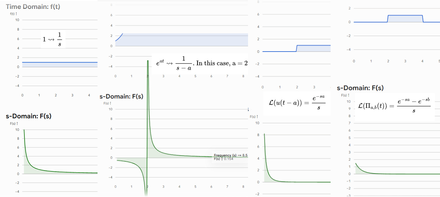
By definition, the Laplace Transform is given by: $\mathcal{L}(1) = \int_{0}^{∞} 1e^{-st}dt = \int_{0}^{∞} e^{-st}dt$

To evaluate this improper integral, we take the limit as the upper bound approaches infinity: $\mathcal{L}\{1\} = \lim_{R \to \infty} \int_{0}^{R} e^{-st} dt$

Compute the definite integral over the finite interval [0, R]: $\int_{0}^{R} e^{-st}dt = \frac{e^{-st}}{-s}\bigg|_{0}^{R} = \frac{e^{-sR}-1}{-s}$

$\int_{0}^{∞} e^{-st}dt = \lim_{R \to ∞}\int_{0}^{R} e^{-st}dt = \lim_{R \to ∞} \frac{e^{-sR}-1}{-s} =[\text{Since s > 0, as R → ∞, } e^{-sR}→ 0] \frac{1}{s}$, this is true only for s > 0.

$\mathcal{L}(1) = \frac{1}{s}$ or $1 \leadsto \frac{1}{s}$. This means that the function f(t) = 1 maps to F(s) = $\frac{1}{s}$$ under the Laplace Transform.

• Laplace Transform of the exponential function $f(t) = e^{at}$

First, we are going to calculate the Laplace Transform of e^atf(t), where f(t) is a function whose Laplace Transform is F(s).

By definition, the Laplace Transform of e^atf(t) is: $\mathcal{L}(e^{at}f(t)) = \int_{0}^{∞} e^{at}f(t)e^{-st}dt =[\text{Simplify the exponentials:}] \int_{0}^{∞} e^{-(s-a)t}f(t)dt$

Notice that this is the exact definition of the standard Laplace transform, except the variable s has been replaced by s − a rovided that s-a > 0, which implies s > a.

$e^{at}f(t) \leadsto F(s-a)$ for s > a, assuming $\int_{0}^{∞} f(t)e^{-st}dt = F(s)$. This result is known as the Exponential Shift Formula. This formula shows that multiplying a function by an exponential term $e^{at}$ in the time domain simply shift its Laplace Transform horizontally by a in the s-domain (from F(s) to F(s -a)).

Consider the specific case where f(t) = 1. Then, $e^{at}·1 = e^{at}\leadsto F(s−a) = \frac{1}{s-a}$ for s > a, since $1 \leadsto \frac{1}{s}$. In other notation, $\mathcal{L}\{e^{at}\} = \mathcal{L}\{e^{at} \cdot 1\} = \frac{1}{s-a} \quad \text{for } s > a$.

• Laplace Transform of the Shifted Unit Step $u(t-a)$

The unit step function u(t) is defined as: u(t) = $\begin{cases} 0, t < 0 \\\ 1, t ≥ 0 \end{cases}$

The unit step function $u(t)$ (often called the Heaviside step function) turns “on” at $t = 0$. A shifted unit step function $u(t-a)$ introduces a delay, turning on at $t = a$ ($a > 0$):

$$u(t-a) = \begin{cases} 0, & t < a \\ 1, & t \ge a \end{cases}$$

Taking the transform: $\mathcal{L}(u(t-a)) = \int_{0}^{∞} e^{-st}u(t-a)dt$

Because the function is 0 for all u(t−a) = 0 for t < a, we can change the limits of integration: $\mathcal{L}(u(t-a)) = \int_{a}^{∞} e^{-st}·1dt = \frac{e^{-st}}{-s}\bigg|_{a}^{∞} = 0-\frac{e^{-sa}}{-s} = \frac{e^{-sa}}{s}$ (s > 0).

Note: $\lim_{t \to ∞}\frac{e^{-st}}{t} = 0$ (since s > 0).

• Laplace Transform of the Window Function $\Pi_{a, b}(t)$

The window function, $\Pi_{a, b}(t)$, also known as the rectangular or boxcar function is “on” between t=a and t=b, and “off” everywhere else. It is defined as: $\Pi_{a, b}(t) = \begin{cases} 1, &a < t < b \\\ 0, &otherwise \end{cases} =[\text{It can be expressed as the difference of two unit step functions}]$

We can express this easily as the difference between two shifted unit step functions: u(t-a) - u(t-b).

$\mathcal{L}(\Pi_{a, b}(t)) = \mathcal{L}(u(t-a)-u(t-b)) =[\text{Using the linearity property of the Laplace transform}] \mathcal{L}(u(t-a)) -\mathcal{L}(u(t-b)) = \frac{e^{-sa}}{s}-\frac{e^{-sb}}{s} = \frac{e^{-sa}-e^{-sb}}{s}$. This result is valid for $s > 0$, ensuring the convergence of the Laplace transform.

Advanced Laplace Transforms

• Laplace Transform of The Dirac Delta function $\delta(t-a)$

The Dirac delta function $\delta(t)$ is not a function in the traditional sense, but rather a “distribution” or “generalized function.” It represents an infinitely sharp, infinitely dense impulse (like a hammer strike in physics or a voltage spike in a circuit).

It is defined conceptually as: $\delta(t-a) = \begin{cases} 0, & t \neq a \\ \infty, & t = a \end{cases}$

It satisfies two fundamental mathematical properties:

1. Normalization. $\int_{-\infty}^{\infty} \delta(t-a) dt = 1$. This means that the total area under the impulse is exactly 1.
2. The Sifting Property: When multiplied by any continuous function $f(t)$ and integrated, the delta function “sifts” out the value of the function at exactly $t = a$. $\int_{-\infty}^{\infty} \delta(t-a)f(t) dt = f(a)$

To find $\mathcal{L}\{\delta(t-a)\}$, we apply the definition of the Laplace transform: $\mathcal{L}\{\delta(t-a)\} = \int_{0}^{\infty} e^{-st}\delta(t-a) dt$

Since the delta function is zero everywhere except at $t = a$ (and assuming $a \ge 0$), we can evaluate the integral simply by plugging $t=a$ into the rest of the integrand (The Sifting Property): $\mathcal{L}\{\delta(t-a)\} = e^{-sa}$

Note: If $a=0$, meaning the impulse happens exactly at $t=0$, then $\mathcal{L}\{\delta(t)\} = e^0 = 1$.

• The Second Shifting Theorem (Time Delay).

When a system is delayed in time, we use the shifted unit step function u(t −a) to represent a function turning “on” at t = a. There are two common scenarios you will encounter.

Case A: The Function and the Step are Shifted Together

Let’s find $\mathcal{L}(f(t-a)u(t-a)), \mathcal{L}(f(t)u(t-a))$

$\mathcal{L}(f(t-a)u(t-a)) = \int_{0}^{∞} e^{-st}f(t-a)u(t-a)dt$

Because $u(t-a) = 0$ for $t < a$, the integral evaluates to zero before $t=a$. We can change our lower limit to $a$ and drop the step function: $= \int_{a}^{\infty} e^{-st}f(t-a) dt = $

Substitution of variables $v = t -a, dv = dt, t = a \leadsto v = 0; t = \infty \leadsto v = \infty$

$= \int_{0}^{∞} e^{-s(v+a)}f(v)dv = \int_{0}^{∞} e^{-sv}e^{-sa}f(v)dv = e^{-sa}\int_{0}^{∞} e^{-sv}f(v)dv = e^{-sa}\mathcal{L}(f(t)) = e^{-sa}F(s)$ where F(s) is the Laplace transform of f(t).

Result: $\boxed{\mathcal{L}\{f(t-a)u(t-a)\} = e^{-sa}F(s)}$

Case B: Only the Step is Shifted

What if we need to transform $\mathcal{L}(f(t)u(t-a))$?

1. The trick is to define a new function g(t-a) = f(t), which allows us to use the result from the first part. This means $g(t) = f(t+a)$.
2. Using the result from Case A: $\mathcal{L}\{g(t-a)u(t-a)\} = e^{-sa}\mathcal{L}\{g(t)\}$
3. Substitute $f(t+a)$ back in for $g(t)$: Result: $\boxed{\mathcal{L}\{f(t)u(t-a)\} = e^{-sa}\mathcal{L}\{f(t+a)\}}$

• Polynomial Examples with Time Delays

Let’s apply the two formulas above to polynomial functions. Recall that the standard transform for a polynomial is $\mathcal{L}\{t^n\} = \frac{n!}{s^{n+1}}$ and the previous result $\mathcal{L}(f(t-a)u(t-a)) = e^{-sa}F(s)$

Example 1: Shifted together (Case A)

Evaluate $\mathcal{L}\{(t-2)^2 u(t-2)\}$. Here, $a=2$ and $f(t) = t^2$.

$$\mathcal{L}\{(t-2)^2 u(t-2)\} = e^{-2s}\mathcal{L}\{t^2\} = e^{-2s}\left(\frac{2!}{s^3}\right) = \frac{2e^{-2s}}{s^3}$$

Example 2: Shifted step only (Case B)

Evaluate $\mathcal{L}\{t^2 u(t-2)\}$.

$\mathcal{L}(t^2u(t-2))$ = [Recall the previous result $\mathcal{L}(f(t)u(t-a)) = e^{-sa}\mathcal{L}(f(t+a))$] $e^{-s·2}\mathcal{L}((t+2)^2) = e^{-2s}\mathcal{L}(t^2+4t+4) =[\text{Using linearity and } \mathcal{L}(t^n) = \frac{n!}{s^{n+1}}] e^{-2s}(\frac{2}{s^3}+\frac{4}{s^2}+\frac{4}{s})$

Bibliography

1. NPTEL-NOC IITM, Introduction to Galois Theory.
2. Algebra, Second Edition, by Michael Artin.
3. LibreTexts, Calculus and Calculus 3e (Apex). Abstract and Geometric Algebra, Abstract Algebra: Theory and Applications (Judson).
4. Field and Galois Theory, by Patrick Morandi. Springer.
5. Michael Penn, and MathMajor.
6. Contemporary Abstract Algebra, Joseph, A. Gallian.
7. YouTube’s Andrew Misseldine: Calculus. College Algebra and Abstract Algebra.
8. MIT OpenCourseWare [18.03 Differential Equations, Spring 2006], YouTube by MIT OpenCourseWare.
9. Calculus Early Transcendentals: Differential & Multi-Variable Calculus for Social Sciences.