Introduction to Fourier Series and Coefficients

Mathematics is the music of reason, James Joseph Sylvester

Introduction to Fourier Series

In this section, we introduce the concept of the Fourier series, a powerful mathematical tool used to represent virtually any periodic function as an infinite sum of simple sine and cosine waves.

This technique is incredibly useful when analyzing physical systems modeled by inhomogeneous second-order linear differential equations of the form: $y'' + ay' + by = f(t)$ where:

• $y(t)$ is the unknown response or behavior of the system (what we want to solve for).
• $f(t)$ is the known forcing function representing an external, periodic push or pull on the system.
• $a$ and $b$ are constants that describe inherent physical characteristics of the system, such as damping (friction) or stiffness (spring constant).

Up to this point, we have often dealt with simple input functions f(t) like pure exponentials, sines, or cosines. While these might seem like very specific and limited cases, they are actually the fundamental building blocks of the mathematical universe. Because of how these equations work, we can build incredibly complex periodic inputs by stacking these simple sine and cosine waves on top of each other.

This is where the true power of linear differential equations shines. Due to the linear nature of the differential equation, we can decompose or break down more complicated, messy inputs f(t) into a neat stack (sums) of simple sine and cosine waves. We then calculate the system's response to each individual wave, and simply add all those individual responses together to get the total system response. This principle is known as superposition and it is indeed a cornerstone in solving linear differential equations.

Fourier Series

A Fourier series allows to write or express any periodic function f(t) (with a period of $2\pi$) as an infinite sum of trigonometric functions. The general form of a Fourier series is given by: $\boxed{f(t) = \frac{a_0}{2} + \sum_{n=1}^\infty [a_ncos(nt)+b_nsin(nt)]}$ where:

• $\frac{a_0}{2}$ is the constant term, representing the average (or “DC”) value of the function over one full period. It shifts the entire wave up or down on the y-axis.
• $a_n$ and $b_n$ (The Fourier Coefficients): These constants represent the amplitudes of the respective cosine and sine terms. They dictate “how much” of each specific wave is needed to build the original function.
• $n$ (The Harmonic Number): This is a positive integer ($1, 2, 3, ...$) that determines the frequency of each term. $n=1$ is the fundamental frequency, $n=2$ is the second harmonic (twice as fast), $n=3$ is the third harmonic, and so on.

Key Takeaway: In a Fourier series representation, each sine and cosine term corresponds to a harmonic of the fundamental frequency. By adding up enough of these high-frequency and low-frequency components, you can perfectly capture the shape of the original periodic function.

Superposition of Solutions

When solving the differential equation $y'' + ay' + by = f(t)$, the principle of superposition acts as our strategic roadmap.

The Rule of Superposition states: If $f(t)$ is composed of a sum of several smaller functions, then the total system response $y(t)$ is simply the sum of the responses to each of those smaller functions.

This gives us a clear, three-step method for solving complex ODEs:

1. Decompose the complicated (or messy) input f(t) into a sum of sines and cosines using its Fourier series.
2. Solve the differential equation to find the particular response for each individual sine and cosine term.
3. Sum all of those individual responses together to obtain the total, overall response y(t).

Mapping Inputs to Responses

The table below illustrates exactly how different components of the Fourier series input translate into specific pieces of the total solution.

Let $y_n^{(s)}(t)$ denote the particular response to a pure $\sin(nt)$ input, and $y_n^{(c)}(t)$ denote the response to a pure $\cos(nt)$ input.

Table of Inputs and Responses

If we can solve the equation for basic inputs like sin(nt) and cos(nt), we have essentially “hacked” the system. This table illustrates the superposition principle: since the differential equation is linear, the response to a sum of inputs is simply the sum of the responses to each input. If we can solve the equation for simple inputs like sin(nt) and cos(nt), we can construct the solution for any periodic input function by adding up the responses corresponding to its Fourier components.

Orthogonality of Sine and Cosine Functions

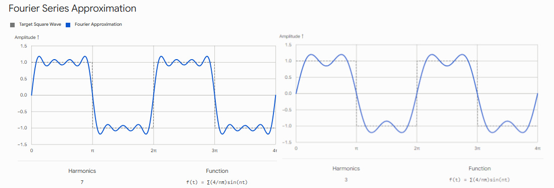
Before diving into how we calculate the coefficients of a Fourier series, we must understand the fundamental property that makes the entire system work: orthogonality.

Definition. Two functions $u(t)$ and $v(t)$, defined on $\mathbb{R}$ and periodic with period $2\pi$, are said to be orthogonal on the interval $[-\pi, \pi]$ if the integral of their product over that interval is zero: $\int_{-\pi}^{\pi} u(t)v(t)dt = 0$

Theorem. Orthogonality of Sines and Cosines. The infinite set of trigonometric functions: $\begin{cases} sin(nt) n = 1, 2, 3, ··· \\\ cos(mt) m = 0, 1, 2, ··· \end{cases}$ is orthogonal on the interval $[-\pi, \pi]$. This means that, for any two distinct functions from this set, the integral of their product over a whole period $[-\pi, \pi]$ is zero:

• $\int_{-\pi}^{\pi} \sin(nt)\sin(mt)dt = 0 \quad (\text{when } n \neq m)$
• $\int_{-\pi}^{\pi} \cos(nt)\cos(mt)dt = 0 \quad (\text{when } n \neq m)$
• $\int_{-\pi}^{\pi} \sin(nt)\cos(mt)dt = 0 \quad (\text{for all } n, m)$

Note on Identical Functions (The Exceptions)

When the functions are identical ($n = m \neq 0$), the integral does not vanish. Instead, it yields exactly half the integration interval: $\int_{-\pi}^{\pi} \sin^2(nt)dt = \int_{-\pi}^{\pi} \cos^2(nt)dt = \pi$

For the special case where $n = 0$: $\int_{-\pi}^{\pi} \cos^2(0 \cdot t)dt = \int_{-\pi}^{\pi} 1^2dt = 2\pi$

Why does this matter? Orthogonality in this context means that the sine and cosine functions are “independent” of each other in a certain sense. In the Fourier series, we decompose a periodic function into a sum of sines and cosines. This property ensures that each Fourier coefficient (associated with a particular sine or cosine function) is independent of the others and can be calculated separately.

Proof of Orthogonality:

Let $U_n(t)$ and $V_m(t)$ be any two functions from the set of sines or cosines, where their frequencies are different ($n \neq m$). We want to prove: $\int_{-\pi}^{\pi} U_n(t)V_m(t)dt = 0$

We begin by recalling that both sine and cosine functions satisfy the standard second-order differential equation for a harmonic oscillator: $U_n''(t) + n^2U_n(t) = 0 \implies U_n''(t) = -n^2U_n(t)$ where $U_n(t)$ can represent either $\sin(nt)$ or $\cos(nt)$.

We are interested in proving that for n ≠ m: $\int_{-π}^{π} U_n(t)V_m(t)dt = 0$

$U_n''(t)V_m(t)$ using integration by parts ($\int u dv = uv - \int v du$):

$\int_{-\pi}^{\pi} U_n''(t)V_m(t)dt = \left[ U_n'(t)V_m(t) \right]_{-\pi}^{\pi} - \int_{-\pi}^{\pi} U_n'(t)V_m'(t)dt$

The boundary term $\left[ U_n'(t)V_m(t) \right]_{-\pi}^{\pi}$ evaluates to zero (periodicity). Because both functions and their derivatives repeat every $2\pi$, their values at $t = \pi$ are identical to their values at $t = -\pi$. Therefore, subtracting the lower bound from the upper bound results in exactly $0$.

With the boundary term gone, we are left with: $\int_{-\pi}^{\pi} U_n''(t)V_m(t)dt = - \int_{-\pi}^{\pi} U_n'(t)V_m'(t)dt$

Substitute the harmonic oscillator identity $U_n''(t) = -n^2U_n(t)$ into the left side, we get the expression: $-n^2\int_{-\pi}^{\pi} U_n(t)V_m(t)dt = - \int_{-\pi}^{\pi} U_n'(t)V_m'(t)dt$

By applying the exact same integration by parts logic to $V_m''(t) = -m^2V_m(t)$, we get a symmetrical equation: $-m^2\int_{-\pi}^{\pi} U_n(t)V_m(t)dt = - \int_{-\pi}^{\pi} U_n'(t)V_m'(t)dt$

Since the right sides of both equations are identical, we can obviously set their left sides equal to each other: $-n^2\int_{-\pi}^{\pi} U_n(t)V_m(t)dt = -m^2\int_{-\pi}^{\pi} U_n(t)V_m(t)dt$

Bring everything to one side and factor out the common integral: $(n^2 - m^2)\int_{-\pi}^{\pi} U_n(t)V_m(t)dt = 0$

Because we defined $n$ and $m$ as two distinct integers ($n \neq m$), we know that $(n^2 - m^2) \neq 0$. Therefore, to satisfy the equation, the integral itself must be zero: $\int_{-\pi}^{\pi} U_n(t)V_m(t)dt = 0 \quad \blacksquare$

Fourier Series and Fourier Coefficients

The Fourier series is a powerful tool that allows us to represent any well-behaved periodic function f(t) as a sum of sine and cosine functions. Specifically, if a function f(t) is periodic with a period of $2\pi$, we can express it as an infinite series involving cosines and sines: $f(t) = \frac{a_0}{2} + \sum_{n=1}^\infty [a_ncos(nt)+b_nsin(nt)]$

The ultimate goal is to determine the Fourier coefficients ($a_0$, $a_n$, and $b_n$). These coefficients act as weights, describing or quantifying exactly how much of each specific sine and cosine harmonic is required to build the overall function $f(t)$

Steps to Determine the Fourier Coefficients

Because the trigonometric functions are orthogonal, we can use a clever “filtering” technique to isolate and solve for each coefficient one by one.

Solve for $a_n$

1. To isolate a specific coefficient $a_n$, we multiply both sides of the Fourier series equation by $\cos(nt)$: $f(t)cos(nt) = \frac{a_0}{2}cos(nt) + \sum_{m=1}^\infty [a_mcos(mt)+b_msin(mt)]cos(nt) = \frac{a_0}{2}cos(nt) + \sum_{m=1}^\infty [a_mcos(mt)cos(nt)+b_msin(mt)cos(nt)]$

2. Next, we integrate both sides over the full period $[-\pi, \pi]$: $\int_{-\pi}^{\pi} f(t)\cos(nt)dt = \frac{a_0}{2}\int_{-\pi}^{\pi} \cos(nt)dt + \sum_{m=1}^\infty \left[ a_m\int_{-\pi}^{\pi}\cos(mt)\cos(nt)dt + b_m\int_{-\pi}^{\pi} \sin(mt)\cos(nt)dt \right]$

3. Because of the orthogonality property, almost every single integral on the right side of the equation evaluates to zero!
   $\int_{-\pi}^{\pi} \cos(nt)dt = 0$, $\int_{-\pi}^{\pi} \sin(mt)\cos(nt)dt = 0$ (for all $m, n$), and $\int_{-\pi}^{\pi} \cos(mt)\cos(nt)dt = 0$ (whenever $m \neq n$)
   The infinite series collapses, and the only term that survives is the one where $m = n$: $\int_{-\pi}^{\pi} f(t)\cos(nt)dt = a_n\int_{-\pi}^{\pi}\cos^2(nt)dt$

4. Since we know that $\int_{-\pi}^{\pi} \cos^2(nt)dt = \pi$, the equation becomes: $\int_{-\pi}^{\pi} f(t)\cos(nt)dt = a_n \cdot \pi$

5. Dividing by $\pi$, we get the formula for $a_n$: $\boxed{a_n = \frac{1}{\pi}\int_{-\pi}^{\pi} f(t)\cos(nt)dt}$

Solve for $b_n$

The process for $b_n$ is identical, except we multiply the original Fourier series by $\sin(nt)$ and integrate. Due to orthogonality, every term vanishes except for the $b_n\sin^2(nt)$ term: $\int_{-\pi}^{\pi} f(t)\sin(nt)dt = b_n\int_{-\pi}^{\pi}\sin^2(nt)dt$

Since we know that $\int_{-\pi}^{\pi} \sin^2(nt)dt = \pi$, the equation becomes: $\int_{-\pi}^{\pi} f(t)\sin(nt)dt = b_n \cdot \pi$

Dividing by $\pi$, we get the formula for $b_n$: $\boxed{b_n = \frac{1}{\pi}\int_{-\pi}^{\pi} f(t)\sin(nt)dt}$

Solve for $a_0$ (The Constant Term)

To find the baseline coefficient $a_0$, we simply integrate the original function $f(t)$ over $[-\pi, \pi]$ without multiplying it by anything: $\int_{-\pi}^{\pi} f(t)dt = \int_{-\pi}^{\pi} \frac{a_0}{2}dt + \sum_{n=1}^\infty \left[ a_n\int_{-\pi}^{\pi} \cos(nt)dt + b_n\int_{-\pi}^{\pi} \sin(nt)dt \right]$

Because the integrals of pure sines and cosines over a full period are zero, the entire infinite sum disappears, leaving: $\int_{-\pi}^{\pi} f(t)dt = \frac{a_0}{2} \int_{-\pi}^{\pi} 1 dt = \frac{a_0}{2}(2\pi) = a_0 \cdot \pi$

Dividing by $\pi$, we get the formula for $a_0$: $\boxed{a_0 = \frac{1}{\pi}\int_{-\pi}^{\pi} f(t)dt}$

$\frac{a_0}{2}$ simply represents the average value of the function $f(t)$ over one period.

Summary

To summarize, if $f(t)$ is periodic with period $2\pi$, its Fourier series is: $f(t) = \frac{a_0}{2} + \sum_{n=1}^\infty \left[ a_n\cos(nt) + b_n\sin(nt) \right]$ where the coefficients are given by Euler’s formulas: $\boxed{a_0 = \frac{1}{\pi}\int_{-\pi}^{\pi} f(t)dt}, \boxed{a_n = \frac{1}{\pi}\int_{-\pi}^{\pi} f(t)\cos(nt)dt}, \text{ and } \boxed{b_n = \frac{1}{\pi}\int_{-\pi}^{\pi} f(t)\sin(nt)dt}$

Bibliography

1. NPTEL-NOC IITM, Introduction to Galois Theory.
2. Algebra, Second Edition, by Michael Artin.
3. LibreTexts, Calculus and Calculus 3e (Apex). Abstract and Geometric Algebra, Abstract Algebra: Theory and Applications (Judson).
4. Field and Galois Theory, by Patrick Morandi. Springer.
5. Michael Penn, and MathMajor.
6. Contemporary Abstract Algebra, Joseph, A. Gallian.
7. YouTube’s Andrew Misseldine: Calculus. College Algebra and Abstract Algebra.
8. MIT OpenCourseWare [18.03 Differential Equations, Spring 2006], YouTube by MIT OpenCourseWare.
9. Calculus Early Transcendentals: Differential & Multi-Variable Calculus for Social Sciences.