Solving Inhomogeneous Systems of ODEs

All warfare is based on deception, Sun tzu, The Art of War

War is a racket. It always has been. It is possibly the oldest, easily the most profitable, surely the most vicious. It is the only one international in scope. It is the only one in which the profits are reckoned in dollars and the losses in lives, Smedley Butler

Inhomogeneous Systems

In the study of differential equations, many real-world problems can be modeled using systems of equations that include external inputs or driving forces. These are known as inhomogeneous (or non-homogeneous) systems. Understanding how to solve such systems is crucial in fields like engineering, physics, and applied mathematics.

We will explore how to solve a system of inhomogeneous differential equations using advanced matrix methods.

The Inhomogeneous System

Consider the following system of first-order linear differential equations: $\begin{cases} x' = ax + by + r_1(t) \\\ y' = cx + dy + r_2(t) \end{cases}$ where:

• x(t) and y(t) are the unknown functions of time t.
• a, b, c, and d are constants coefficients.
• $r_1(t)$ and $r_2(t)$ are known functions representing external inputs, forces, or sources acting on the system.

Matrix Representation

This system can be written in matrix form as: $\vec{X'} = A\vec{X}+\vec{r}(t)$ where:

• A = $(\begin{smallmatrix}a & b\\\ c & d\end{smallmatrix})$ is the constant coefficient matrix.
• $\vec{X} = (\begin{smallmatrix}x\\\ y\end{smallmatrix})$ is the state vector of unknown functions.
• $\vec{r}(t)= (\begin{smallmatrix}r_1(t)\\\ r_2(t)\end{smallmatrix})$ is the vector of nonhomogeneous terms. It represents the external inputs or forces acting on the system.

General Solution of the Inhomogeneous System

Theorem. General Solution. The general solution to the inhomogeneous system $\vec{X'} = A\vec{X}+\vec{r}(t)$ is given by: $\vec{x_{gen}} = \vec{x_c}+\vec{x_p}$ where:

1. $\vec{x_c}$ is the complementary (or homogeneous) solution. This is the the general solution to the associated homogeneous system, $\vec{X'} = A\vec{X}$, where $\vec{r}(t)=0$. This gives us the complementary solution $\vec{x_c}$, which is based on the eigenvalues and eigenvectors of the matrix A. It represents the natural, unforced behavior of the system (without external inputs) or transient state of the system.
2. $\vec{x_p}$ is any single solution that satisfies the full inhomogeneous system. A solution that satisfies the full inhomogeneous system, including the non-homogeneous term $\vec{r}(t)$. It accounts for the system’s specific response to the external inputs.

Therefore, the general solution is the sum of the complementary and particular solutions: $\vec{x_{gen}} = \vec{x_c}+\vec{x_p}$.

Proof:

Let $\vec{x_c},\vec{x_p}$ be complementary and particular solution that satisfies: $\vec{X'} = A\vec{X},\text{ and} \vec{X'} = A\vec{X}+\vec{r}(t)$ respectively.

We propose that the general solution can be expressed as: $\vec{x_{gen}} = \vec{x_c}+\vec{x_p}$

$\vec{x_{gen}} = \vec{x'_c}+\vec{x'_p}$

Since $\vec{x_c}$​ is a solution to the inhomogeneous equation, and $\vec{x_p}$ is a solution to the homogeneous associated equation, we get: $\vec{x_{gen}} = $A\vec{x_c}+A\vec{x_p}+\vec{r}(t)$

Factor out A $\vec{x_{gen}} = A(\vec{x_c}+\vec{x_p})+\vec{r}(t) = A\vec{x_{gen}}+\vec{r}(t)$ which shows that $\vec{x_{gen}}$ satisfies the inhomogeneous differential system.

Real-World Application: The Mixing Problem

To find the particular solution $\vec{x}_p(t)$, we use the Variation of Parameters method.

We assume the particular solution has the same structure as the complementary solution, but we allow the constants to vary over time. If the fundamental matrix of the homogeneous system is $X(t)$, we assume: $\vec{x}_p(t) = X(t)\vec{v}(t)$ where $\vec{v}(t) = \begin{pmatrix} v_1(t) \\ v_2(t) \end{pmatrix}$ is a vector of unknown functions to be determined.

Let’s substitute this into the non-homogeneous equation $\vec{x}_p' = A\vec{x}_p + \vec{r}(t)$.

First, differentiate $\vec{x}_p(t)$ using the product rule: $\vec{x}_p' = X'(t)\vec{v}(t) + X(t)\vec{v}'(t)$

Substitute this into the left side ($\vec{x}_p' = A\vec{x}_p + \vec{r}(t)$), and $\vec{x}_p(t) = X(t)\vec{v}(t)$ into the right side: $X'(t)\vec{v}(t) + X(t)\vec{v}'(t) = AX(t)\vec{v}(t) + \vec{r}(t)$

Recall that because every column of $X(t)$ is a solution to the homogeneous equation, $X'(t) = AX(t)$. Therefore, the $X'(t)\vec{v}(t)$ and $AX(t)\vec{v}(t)$ terms cancel out, and we get: $X(t)\vec{v}'(t) = \vec{r}(t)$

Solving for $\vec{v}'(t)$ by multiplying by the inverse fundamental matrix $X^{-1}(t)$: $\vec{v}'(t) = X^{-1}(t)\vec{r}(t)$

Integrating this gives $\vec{v}(t) = \int X^{-1}(t)\vec{r}(t) dt$.

Finally, substituting $\vec{v}(t)$ back into our initial assumption gives the Variation of Parameters Formula: $\boxed{\vec{x}_p(t) = X(t) \int X^{-1}(t)\vec{r}(t) dt}$ (Note: We don’t need to add constants of integration here, as they are already accounted for in the complementary solution $\vec{x}_c$.) ​

Example: Mixing Problem

Consider a system involving two interconnected tanks, each with a capacity of 1 liter. The tanks are labeled Tank 1 and Tank 2. They are connected by pipes that allow liquid to flow between them at specified rates. We are interested in determining how the amount of salt in each tank changes over time.

As it is illustrated, 2 indicates that the liquid flows from the right tank, 2, to the left tank, 1; 3: the liquid flows from the left tank 1 to the right tank 2. Both tanks have a external inflow port to fill in the container and only the one on the right, the 2 container, have a an outflow (drain) to release its content. The flow rates are measured in liters/hour. x and y describes the amount of salt (in grams) in tank 1 and 2 respectively.

Flow Rates:

• Tank 1 Inflows: Receives 2 L/hr from Tank 2 (it is coming in (2 → 1)). It also receives an external inflow of 1 L/hr containing a salt concentration of $5e^{-t}$ g/L.
• Tank 1 Outflows: Pumps 3 L/hr into Tank 2 (3 is coming out (1 → 3)). Total volume stays constant at 1L: 2+1 in, 3 out.
• Tank 2 Inflows: Receives 3 L/hr from Tank 1. It also receives an external inflow of 1 L/hr of pure water (0 g/L).
• Tank 2 Outflows: Pumps 2 L/hr back to Tank 1, and drains 2 L/hr out of the system entirely. Total volume stays constant at 1L: 3+1 in, 2+2 out.

Deriving the Differential Equations

Using the principle $\text{Rate of Change} = \text{Rate In} - \text{Rate Out}$:

• Rate of change of salt in Tank 1: $x' = \left( 2y + 1(5e^{-t}) \right) - (3x) = -3x + 2y + 5e^{-t}$.
• Rate of change of salt in Tank 2: $y' = \left( 3x + 1(0) \right) - (2y + 2y) = 3x - 4y$.

Thus, we have the system:

$\begin{cases} x' = -3x +2y + 5e^{-t} \\\ y' = 3x -4y + 0 \end{cases}$ where x(t) represents the amount of salt in tank 1, and y(t) represents the amount of salt in tank 2 (Refer to Figure vi for a visual representation and aid in understanding it).

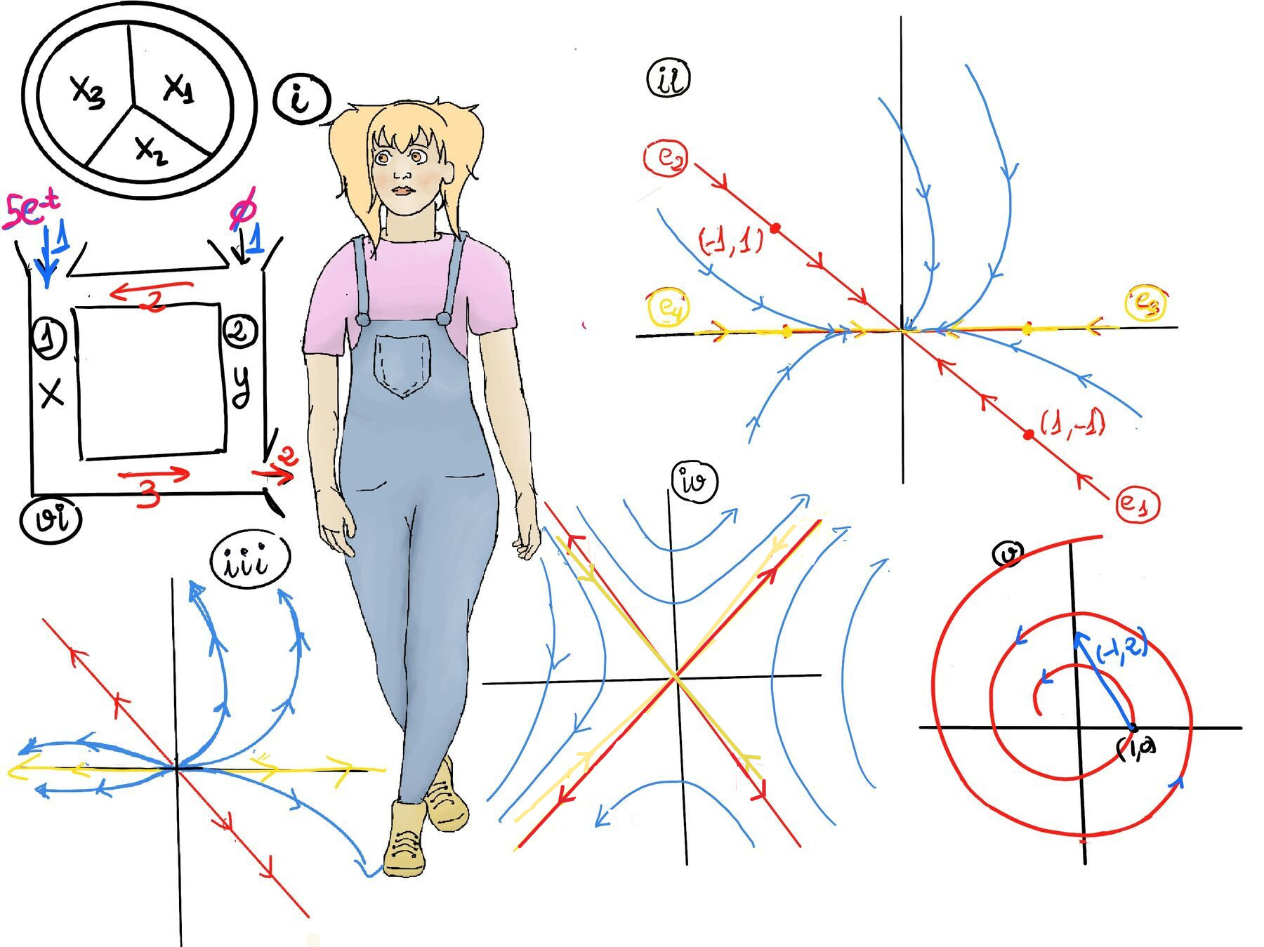
This is an inhomogeneous system. This system can be written in matrix form as: $\vec{X'} = A\vec{X} + \vec{r}(t) = (\begin{smallmatrix}-3 & 2\\\ 3 & -4\end{smallmatrix})\vec{X}+(\begin{smallmatrix}5e^{-t}\\\ 0\end{smallmatrix})$

Solving the Mixing Problem

Step 1. Solve the Homogeneous System

To solve this, we need to find the eigenvalues and eigenvectors of the matrix A = $(\begin{smallmatrix}-3 & 2\\\ 3 & -4\end{smallmatrix})$

The characteristic equation is obtained from: $\det(A - \lambda I) = 0$ where I is the identity matrix.

So: $det(\begin{smallmatrix}-3-λ & 2\\\ 3 & -4-λ\end{smallmatrix}) = 0$

Expanding the determinant: $\lambda^2 + 7\lambda + 12 - 6 = \lambda^2 + 7\lambda + 6 = 0$

$(\lambda + 1)(\lambda + 6) = 0 \implies \lambda_1 = -1, \quad \lambda_2 = -6$

Find the Eigenvectors:

For $\lambda_1 = -1$, we solve: $\begin{pmatrix} -3-(-1) & 2 \\ 3 & -4-(-1) \end{pmatrix} = \begin{pmatrix} -2 & 2 \\ 3 & -3 \end{pmatrix} \implies -2v_x + 2v_y = 0 \implies v_x = v_y$

Eigenvector: $\vec{v}_1 = \begin{pmatrix} 1 \\ 1 \end{pmatrix}$

For $\lambda_2 = -6$, we solve: $\begin{pmatrix} -3-(-6) & 2 \\ 3 & -4-(-6) \end{pmatrix} = \begin{pmatrix} 3 & 2 \\ 3 & 2 \end{pmatrix} \implies 3v_x + 2v_y = 0 \implies v_x = -\frac{2}{3}v_y$

Eigenvector: $\vec{v}_2 = \begin{pmatrix} -2 \\ 3 \end{pmatrix}$

The complementary solution (general solution to the homogeneous system) is: $\vec{x}_c(t) = c_1 e^{-t} \begin{pmatrix} 1 \\ 1 \end{pmatrix} + c_2 e^{-6t} \begin{pmatrix} -2 \\ 3 \end{pmatrix}$

Step 2: Find the Particular Solution ($\vec{x}_p$)

1. We assume the particular solution is of the form: $\vec{x_p} = v_1(t)\vec{x_1}+v_2(t)\vec{x_2}$ where $\vec{x_1} = (\begin{smallmatrix}e^{-t}\\\ e^{-t}\end{smallmatrix})$ and $\vec{x_2} = (\begin{smallmatrix}-2e^{-6t}\\\ 3e^{-6t}\end{smallmatrix})$ are the solutions to the homogeneous system, $\vec{v} = (\begin{smallmatrix}v_1(t)\\\ v_2(t)\end{smallmatrix})$
   Thus, $\vec{x_p}(t) = (\begin{smallmatrix}e^{-t} & -2e^{-6t}\\\ e^{-t} & 3e^{-6t}\end{smallmatrix})(\begin{smallmatrix}v_1(t)\\\ v_2(t)\end{smallmatrix}) = X(\begin{smallmatrix}v_1(t)\\\ v_2(t)\end{smallmatrix}) = X(t)\vec{v}(t)$ and $X(t) = \begin{pmatrix} e^{-t} & -2e^{-6t} \\ e^{-t} & 3e^{-6t} \end{pmatrix}$
2. Compute the determinant of $X(t)$ (the Wronskian): $\det(X(t)) = (e^{-t})(3e^{-6t}) - (-2e^{-6t})(e^{-t}) = 3e^{-7t} + 2e^{-7t} = 5e^{-7t}$
3. Find the inverse matrix $X^{-1}(t)$: $X^{-1}(t) = \frac{1}{5e^{-7t}} \begin{pmatrix} 3e^{-6t} & 2e^{-6t} \\ -e^{-t} & e^{-t} \end{pmatrix} = \begin{pmatrix} \frac{3}{5}e^{t} & \frac{2}{5}e^{t} \\ -\frac{1}{5}e^{6t} & \frac{1}{5}e^{6t} \end{pmatrix}$
   $X^{-1}(t) = \frac{1}{det(X(t))}(\begin{smallmatrix}x_{22}(t) & -x_{12}(t)\\\ -x_{21}(t) & x_{11}(t)\end{smallmatrix}) = \frac{1}{5e^{-7t}} (\begin{smallmatrix}3e^{-6t} & 2e^{-6t}\\\ -e^{-t} & e^{-t}\end{smallmatrix})$
4. Now, compute $\vec{v}'(t) = X^{-1}(t)\vec{r}(t)$: $\vec{v}'(t) = \begin{pmatrix} \frac{3}{5}e^{t} & \frac{2}{5}e^{t} \\ -\frac{1}{5}e^{6t} & \frac{1}{5}e^{6t} \end{pmatrix} \begin{pmatrix} 5e^{-t} \\ 0 \end{pmatrix} = \begin{pmatrix} \left(\frac{3}{5}e^{t}\right)(5e^{-t}) + 0 \\ \left(-\frac{1}{5}e^{6t}\right)(5e^{-t}) + 0 \end{pmatrix} = \begin{pmatrix} 3 \\ -e^{5t} \end{pmatrix}$
5. Integrate to find $\vec{v}(t)$: $\vec{v}(t) = \begin{pmatrix} \int 3 \, dt \\ \int -e^{5t} \, dt \end{pmatrix} = \begin{pmatrix} 3t \\ -\frac{1}{5}e^{5t} \end{pmatrix}$
6. Multiply by $X(t)$ to find $\vec{x}_p$: $\vec{x}_p(t) = \begin{pmatrix} e^{-t} & -2e^{-6t} \\ e^{-t} & 3e^{-6t} \end{pmatrix} \begin{pmatrix} 3t \\ -\frac{1}{5}e^{5t} \end{pmatrix} = \begin{pmatrix} 3te^{-t} + \frac{2}{5}e^{-t} \\ 3te^{-t} - \frac{3}{5}e^{-t} \end{pmatrix} = e^{-t} \begin{pmatrix} 3t + \frac{2}{5} \\ 3t - \frac{3}{5} \end{pmatrix}$

Step 3: General Solution

The general solution to the inhomogeneous system is the sum of the complementary and particular solutions: $\vec{x}_{\text{gen}} = \vec{x}_c + \vec{x}_p$: $\vec{X}(t) = c_1 e^{-t} \begin{pmatrix} 1 \\ 1 \end{pmatrix} + c_2 e^{-6t} \begin{pmatrix} -2 \\ 3 \end{pmatrix} + e^{-t} \begin{pmatrix} 3t + \frac{2}{5} \\ 3t - \frac{3}{5} \end{pmatrix}$

We can group the $e^{-t}$ terms together for an even cleaner final answer: $\boxed{\vec{X}(t) = e^{-t} \begin{pmatrix} c_1 + 3t + \frac{2}{5} \\ c_1 + 3t - \frac{3}{5} \end{pmatrix} + c_2 e^{-6t} \begin{pmatrix} -2 \\ 3 \end{pmatrix}}$

The general solution provides the amounts of salt x(t) and y(t) in tanks 1 and 2 at time t, with constant $c_1$ and $c_2$ determined by initial conditions.

Analytical Insight (Resonance): Notice the presence of $t e^{-t}$ in our final solution. This occurs because the external input $5e^{-t}$ operates at the exact same exponential “frequency” as one of the natural eigenvectors ($e^{-t}$) of the tanks. Mathematically, this is analogous to resonance in a mechanical system! Over time, the $e^{-6t}$ term vanishes quickly, and the system is entirely dominated by the $3te^{-t}$ washout curve.

Example 2: Polynomial Inputs and Undetermined Coefficients

Let’s explore another example that demonstrates a powerful alternative method when the non-homogeneous term $\vec{r}(t)$ is mathematically simple (like a polynomial).

Solve the following system: $\begin{cases} x' = -2x +y\\\ y' = x -2y + 3t \end{cases}$

Step 1: Write the System in Matrix Form

We can express the system in matrix form as: $\vec{X'} = A\vec{X} + \vec{r}(t)$ where:

$\vec{X} = (\begin{smallmatrix}x\\\ y\end{smallmatrix}), A = (\begin{smallmatrix}-2 & 1\\\ 1 & -2\end{smallmatrix}), \vec{r}(t) = (\begin{smallmatrix}0\\\ 3t\end{smallmatrix})$

Step 2. Solve the Homogeneous System

First, we find the eigenvalues of $A$ by solving the characteristic equation: $\det(A - \lambda I) = \det \begin{pmatrix} -2-\lambda & 1 \\ 1 & -2-\lambda \end{pmatrix} = (-2-\lambda)^2 - 1 = 0$

Expand and solve, $(\lambda+2-1)(\lambda+2+1) = (\lambda+1)(\lambda+3) = 0 \implies \lambda_1 = -1, \quad \lambda_2 = -3$

Next, we find the corresponding eigenvectors:

• For $\lambda_1 = -1$, we solve: $(A + I)\vec{v}_1 = \begin{pmatrix} -1 & 1 \\ 1 & -1 \end{pmatrix} \begin{pmatrix} v_{1x} \\ v_{1y} \end{pmatrix} = \begin{pmatrix} 0 \\ 0 \end{pmatrix} \implies -v_{1x} + v_{1y} = 0 \implies v_{1x} = v_{1y}=[\text{For simplicity}] 1$.
  Then, $\vec{v}_1 = \begin{pmatrix} 1 \\ 1 \end{pmatrix}$

• For $\lambda_2 = -3$: $(A + 3I)\vec{v}_2 = \begin{pmatrix} 1 & 1 \\ 1 & 1 \end{pmatrix} \begin{pmatrix} v_{2x} \\ v_{2y} \end{pmatrix} = \begin{pmatrix} 0 \\ 0 \end{pmatrix} \implies v_{2x} + v_{2y} = 0 \implies v_{2x} = -v_{2y}$. Let $v_{2x} = 1$.
  $\vec{v}_2 = \begin{pmatrix} 1 \\ -1 \end{pmatrix}$

The complementary solution is: $\vec{x}_c(t) = c_1 e^{-t} \begin{pmatrix} 1 \\ 1 \end{pmatrix} + c_2 e^{-3t} \begin{pmatrix} 1 \\ -1 \end{pmatrix}$

Step 3: Finding the Particular Solution (Variation of Parameters)

1. To use variation of parameters, we build the fundamental matrix $X(t)$: $X(t) = \begin{pmatrix} e^{-t} & e^{-3t} \\ e^{-t} & -e^{-3t} \end{pmatrix}$
2. The Wronskian is $\det(X(t)) = -2e^{-4t}$, giving the inverse matrix: $X^{-1}(t) = \frac{1}{-2e^{-4t}} \begin{pmatrix} -e^{-3t} & -e^{-3t} \\ -e^{-t} & e^{-t} \end{pmatrix}$
   Since det(X(t)) ≠ 0 for all t, X(t) is invertible. For a 2 x 2 matrix X = $(\begin{smallmatrix}a & b\\\ c & d\end{smallmatrix})$, the inverse is $\frac{1}{det(X)}(\begin{smallmatrix}d & -b\\\ -c & a\end{smallmatrix})$
3. We calculate $\vec{v}'(t) = X^{-1}(t)\vec{r}(t)$: $\vec{v}'(t) = \frac{1}{-2e^{-4t}} \begin{pmatrix} -e^{-3t} & -e^{-3t} \\ -e^{-t} & e^{-t} \end{pmatrix} \begin{pmatrix} 0 \\ 3t \end{pmatrix} = \frac{1}{-2e^{-4t}} \begin{pmatrix} -3te^{-3t} \\ 3te^{-t} \end{pmatrix} = \begin{pmatrix} \frac{3}{2}te^{t} \\ -\frac{3}{2}te^{3t} \end{pmatrix}$
4. To find $\vec{v}(t)$, we must integrate these terms. Because of the $t$ multiplied by the exponentials, both components require Integration by Parts ($\int u \, dv = uv - \int v \, du$).
   Use integration by parts u = t, dv = $e^tdt$. Then du = dt, v = $e^t$. $\int te^tdt = te^t -\int e^tdt = te^t-e^t + C$
   $\int t e^t dt = te^t - e^t$
   Use integration by parts u = t, dv = e^3tdt. Then du = dt, v = $\frac{e^{3t}}{3}$
   $\int te^{3t}dt = t\frac{e^{3t}}{3} -\int \frac{e^{3t}}{3}dt = \frac{te^{3t}}{3} -\frac{e^{3t}}{9} + C$
   $\int t e^{3t} dt = \frac{t e^{3t}}{3} - \frac{e^{3t}}{9}$
   Applying these rules gives: $\vec{v}(t) = \begin{pmatrix} \frac{3}{2}(te^t - e^t) \\ -\frac{1}{2}te^{3t} + \frac{1}{6}e^{3t} \end{pmatrix}$

Finally, multiplying $\vec{x}_p = X(t)\vec{v}(t)$ and simplifying everything down yields the particular solution:

$$\vec{x}_p(t) =\begin{pmatrix} e^{-t} & e^{-3t} \\ e^{-t} & -e^{-3t} \end{pmatrix} \begin{pmatrix} \frac{3}{2}(te^t - e^t) \\ -\frac{1}{2}te^{3t} + \frac{1}{6}e^{3t} \end{pmatrix} = \begin{pmatrix} t - \frac{4}{3} \\ 2t - \frac{5}{3} \end{pmatrix}$$

Step 4: The Alternative (and Better!) Method: Undetermined Coefficients

While Variation of Parameters is mathematically guaranteed to work, it required us to compute an inverse matrix involving exponentials, perform two rounds of integration by parts, and carefully expand and cancel terms.

When the non-homogeneous term $\vec{r}(t)$ is a simple polynomial, exponential, or sine/cosine wave, we can skip the calculus entirely using the Method of Undetermined Coefficients.

Since $\vec{r}(t) = \begin{pmatrix} 0 \\ 3 \end{pmatrix}t$ is a linear polynomial vector, we can logically “guess” that the particular solution will share the same structure: $\vec{x}_p(t) = \vec{a}t + \vec{b}$ where $\vec{a}$ and $\vec{b}$ are constant vectors we need to determine.

Because $\vec{a}$ and $\vec{b}$ are constants, the derivative is simply: $\vec{x}_p'(t) = \vec{a}$

Substitute our guess into the original differential equation $\vec{x}' = A\vec{x} + \vec{r}(t)$: $\vec{a} = A(\vec{a}t + \vec{b}) + \begin{pmatrix} 0 \\ 3 \end{pmatrix}t$

Next, we distribute the matrix $A$ and group the $t$ terms and the constant terms together: $\vec{a} = \left( A\vec{a} + \begin{pmatrix} 0 \\ 3 \end{pmatrix} \right)t + A\vec{b}$

For this equation to be true for all time $t$, the coefficients on both sides must match exactly.

Equation 1 $(\star)$. Match the $t$ terms: $\vec{0} = A\vec{a} + \begin{pmatrix} 0 \\ 3 \end{pmatrix}$
Equation 2 $(\star)$. Match the constants: $\vec{a} = A\vec{b}$

Now we just need to solve these two simple algebraic equations!

From equation 1, we isolate $\vec{a}$: $A\vec{a} = \begin{pmatrix} 0 \\ -3 \end{pmatrix} \implies \vec{a} = A^{-1}\begin{pmatrix} 0 \\ -3 \end{pmatrix}$

Using the standard $2\times 2$ inverse formula, we can easily get $A^{-1} = \frac{1}{3}\begin{pmatrix} -2 & -1 \\ -1 & -2 \end{pmatrix}$, so $\vec{a} = \frac{1}{3}\begin{pmatrix} -2 & -1 \\ -1 & -2 \end{pmatrix} \begin{pmatrix} 0 \\ -3 \end{pmatrix} = \frac{1}{3} \begin{pmatrix} 3 \\ 6 \end{pmatrix} = \begin{pmatrix} 1 \\ 2 \end{pmatrix}$

Now use equation 2 to solve for $\vec{b}$: $\vec{b} = A^{-1}\vec{a} = \frac{1}{3}\begin{pmatrix} -2 & -1 \\ -1 & -2 \end{pmatrix} \begin{pmatrix} 1 \\ 2 \end{pmatrix} = \frac{1}{3} \begin{pmatrix} -4 \\ -5 \end{pmatrix} = \begin{pmatrix} -4/3 \\ -5/3 \end{pmatrix}$

Putting it all together into our initial guess $\vec{x}_p = \vec{a}t + \vec{b}$: $\vec{x}_p(t) = \begin{pmatrix} 1 \\ 2 \end{pmatrix}t + \begin{pmatrix} -4/3 \\ -5/3 \end{pmatrix} = \begin{pmatrix} t - \frac{4}{3} \\ 2t - \frac{5}{3} \end{pmatrix}$. This particular solution matches the one found earlier.

Step 4. Write the General Solution

Combining this with the complementary solution from Step 2, the final general solution is: $\boxed{\vec{x}(t) = \vec{x_h}(t)+\vec{x_p}(t) = c_1e^{-t}(\begin{smallmatrix}1\\\ 1\end{smallmatrix}) + c_2e^{-3t}(\begin{smallmatrix}1\\\ -1\end{smallmatrix}) + (\begin{smallmatrix}t-\frac{4}{3}\\\ 2t -\frac{5}{3}\end{smallmatrix})}$. This is the general solution to the original system.

Bibliography

1. NPTEL-NOC IITM, Introduction to Galois Theory.
2. Algebra, Second Edition, by Michael Artin.
3. LibreTexts, Calculus and Calculus 3e (Apex). Abstract and Geometric Algebra, Abstract Algebra: Theory and Applications (Judson).
4. Field and Galois Theory, by Patrick Morandi. Springer.
5. Michael Penn, and MathMajor.
6. Contemporary Abstract Algebra, Joseph, A. Gallian.
7. YouTube’s Andrew Misseldine: Calculus. College Algebra and Abstract Algebra.
8. MIT OpenCourseWare [18.03 Differential Equations, Spring 2006], YouTube by MIT OpenCourseWare.
9. Calculus Early Transcendentals: Differential & Multi-Variable Calculus for Social Sciences.