Second-Order Linear Differential Equations. Homogeneous vs. Inhomogeneous

The essence of mathematics is not to make simple things complicated, but to make complicated things simple, S. Gudder

I’d far rather be happy than right any day, Douglas Adams, The Hitchhiker’s Guide to the Galaxy.

Second-order Linear Homogeneous ODE’s

Second-order linear ordinary differential equations (ODEs) are the workhorses of mathematical modeling in the physical sciences. They govern everything from the rhythmic sweep of a clock pendulum to the behavior of alternating current circuits, describing systems where acceleration or rate of change depends linearly on both position and velocity (on both the quality and its derivatives).

Second-Order Linear Homogeneous ODEs

Definition. AA second-order linear homogeneous ODE is any differential equation that can be written in the standard form: $y'' + p(x)y' + q(x)y = 0$ where:

• y = y(x) is the unknown function of x we want to solve for.
• $y'$ and $y''$ are its first and second derivatives with respect to $x$, respectively.
• $p(x)$ and $q(x)$ are coefficient functions that can be continuous variables or simple constants.

Breaking Down the Terminology

• Linear: The dependent variable $y$ and its derivatives must only appear to the first power. There can be no nonlinear operations applied to them (such as squares $y^2$, cubes $y^3$, or other nonlinear expressions $\sin(y)$, or $\sqrt{y'}$), and they cannot be multiplied together (such as $y \cdot y'$).

• Homogeneous: The right-hand side of the equation evaluates strictly to zero. This signifies a passive system, indicating that there are no external forcing functions —one evolving completely under its own internal mechanics with absolutely no external forces pushing or pulling on it.

Inhomogeneous Second-Order Linear ODEs

When an external force acts upon our system, the right-hand side is no longer zero. The equation becomes inhomogeneous (or nonhomogeneous): $y'' + p(x)y' + q(x)y = f(x)$

An inhomogeneous second-order linear differential equation is a differential equation of the form: y'' + p(x)y' + q(x)y = f(x) where:

• y is the unknown function of x.
• y’ and y’’ are the first and second derivative of y with respect to x, respectively.
• f(x), p(x) and q(x) are given functions of x.
• f(x) is called the input, forcing term, driving term, or sometimes the input signal.

Our objective shifts to finding the total system response (or output), $y(x)$, under the influence of this external input.

Solving the Inhomogeneous Equation

Solving an inhomogeneous equation requires a beautifully simple additive strategy combining natural behavior with forced behavior:

1. Find the Complementary Solution ($y_c$). We temporarily turn off the external force ($f(x) = 0$) and solve the associated, reduced homogeneous equation.
   The resulting solution is the complementary solution: $y_c(x) = c_1y_1(x) + c_2y_2(x)$ where $y_1$ and $y_2$ are linearly independent solutions of the homogeneous equation and $c_1 and $c_2 are arbitrary constants determined by initial or boundary conditions.
   Linear independence means that one solution cannot be expressed as a scalar multiple of the other. The Wronskian $W(y_1, y_2)$ is non-zero if $y_1$ and $y_2$ are linearly independent on the interval of interest.
   This captures the system’s natural, unforced behavior dictated entirely by its internal properties.

2. Find a Particular Solution ($y_p$). We turn the forcing term back on and find any single, specific function $y_p(x)$ that satisfies the full equation. This particular solution satisfies the inhomogeneous equation, contains no arbitrary constants and models how the system directly responds to the external driving force.

3. Synthesize the Full General Solution. By the Principle of Superposition, the complete general solution is simply the sum of both components: $y(x) = y_c(x) + y_p(x) = c_1y_1(x) + c_2y_2(x) + y_p(x)$ where:
   ($\star$) $y_p(x)$ is any particular solution to the inhomogeneous equation. It represents a specific solution that responds to the forcing term f(x) (it models the system’s response directly due to the external input).
   ($\star$) $y_c(x) = c_1y_1(x) + c_2y_2(x)$ is the general solution to the associated homogeneous equation. It accounts for the behavior of the system without the forcing term f(x). It represents the system’s natural behavior without external forcing or input.
   ($\star$) By combining these, we capture all possible solutions to the inhomogeneous equation.

Real-World Physical Applications

The exact same mathematical structure mirrors different corners of physical reality. Let’s look at the two most famous mechanical and electrical examples. Specifically, we will discuss:

• Application A: The Mechanical Spring-Mass-Dashpot System

This setup models structural vibrations, car suspensions, or seismic building dampening.

The mechanical system is governed by Newton’s Second Law ($\sum F = mx''$), which balances four distinct physical forces: $mx'' + bx' + kx = f(t)$ where:

m: Mass of the object (in kilograms).
b: Damping coefficient (in kilograms per second), related to the dashpot’s resistance.
k: Spring constant, representing the stiffness of the spring. $kx$ is the restoring force. Hooke’s Law for the spring; pulls the mass back toward equilibrium.
x(t): Displacement of the mass from its equilibrium position at time t.
f(t): External or driving force applied to the system (in newtons). The system is said to be forced or influenced by an external force when f(t) ≠ 0, and passive or free when f(t) = 0, meaning that the system evolves solely based on its initial conditions and inherent properties.

mx’’ (inertia term) represents the mass’s resistance to acceleration (Newton’s second law); bx’ (damping term) accounts for the energy loss due to friction or resistance in the dashpot; kx (spring term) represents the restoring force exerted by the spring, proportional to the displacement x; f(t) (external force) is an input function that drives the system, such as an applied push or pull.

Applications: Mechanical engineering (design of suspension system in vehicles), civil engineering (analysis of building responses to earthquakes), and physics (study of oscillatory motion and vibrations).

• Simple Electrical Circuit (RLC Circuit). Switching fields entirely, an RLC circuit guides alternating currents in radios, filters, and power supplies.

A Resistor (R) provides resistance to the flow of current.
An Inductor (L) opposes changes in current due to its magnetic field.
A Capacitor (C) stores electrical energy in an electric field.
A Voltage source ε(t) supplies electromotive force (EMF), which can be constant or time-varying.

According to Kirchhoff’s Voltage Law (KVL), the total loop voltage drop across the components must equal the electromotive forcing voltage $\mathcal{E}(t)$ supplied by the source: $V_L + V_R + V_C = \mathcal{E}(t)$.

Substituting the characteristic electrical properties of each component gives us: $L\frac{di}{dt} + Ri + \frac{q}{C} = \mathcal{E}(t)$ where:

i(t) is the electrical current flowing through the circuit
q(t) is the amount of electric charge stored in the capacitor. Relationship: $\frac{dq}{dt} = i(t)$, meaning the rate of flow of electric charge (dq/dt) with respect to time is equal to the current (i).

Voltage Drops Across Circuit Components:

1. Inductor (L): The voltage drop across an inductor is proportional to the rate of change of current flowing through it: V_L = L * di/dt, where i is the current, di/dt represents the rate of change of current, and t is time.
2. Resistor (R): Following Ohm’s Law, the voltage drop across a resistor is proportional to the current flowing through it: V_R = R * i(t).
3. Capacitor (C): The voltage drop across a capacitor is proportional to the charge stored on its plates: V_C = q/C, where q is the charge of the capacitor and C is the capacitance, a measure of the capacitor’s ability to store charge.
4. Voltage source (ε(t)): The voltage source provides the driving electromotive force (EMF) for the circuit, which can be constant or time-varying, influencing the circuit’s response (Refer to Figure 5 for a visual representation and aid in understanding it).

Deriving the Differential Equation

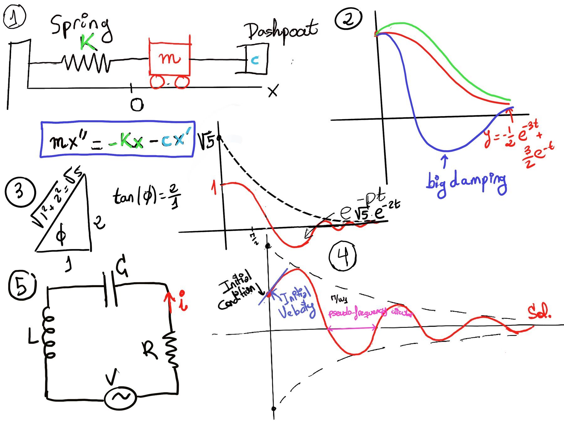
Therefore, $\frac{dq}{dt} = i$ and applying KVL to the RLC circuit gives us the equation: $V_L + V_R + V_C = ε(t) ↭ L\frac{di}{dt}+Ri+\frac{q}{C} = ε(t)$. Differentiating this equation gives: $L\frac{d^2i}{dt^2}+R\frac{di}{dt} + \frac{i}{C} = ε'(t)$ ↭[Notation] $\boxed{Li’’ + Ri’ + \frac{i}{C} = ε’(t)}. This equation governs the flow of current in the circuit in response to an applied voltage ε(t).

Notice the beautiful mathematical isomorphism here. A mechanical engineer and an electrical engineer are solving the exact same calculus problem. Mass ($m$) behaves exactly like Inductance ($L$) (both represent physical inertia). Damping ($b$) behaves exactly like Resistance ($R$) (both represent energy dissipation). Spring Stiffness ($k$) behaves exactly like Reciprocal Capacitance ($\frac{1}{C}$) (both represent potential energy storage).

General Solution to the Inhomogeneous Equation

An inhomogeneous second-order linear differential equation is an equation of the form: $y'' + p(x)y' + q(x)y = f(x)$.

We can express this equation more concisely using a linear differential operator L. Let $L = D^2 + pD + q$, or in full notation: $L = \frac{d^2}{dx^2} + p(x)\frac{d}{dx} + q(x)$ be the differential operator, so our inhomogeneous second-order linear differential equation becomes: $Ly = f(x)$, and the associated homogeneous equation is: Ly = 0.

The general solution to the inhomogeneous equation $Ly = f(x)$ is: $y(x) = y_p(x) + y_c(x) = y_p(x) + c_1y_1(x) + c_2y_2(x)$ where:

• $y_c(x) = c_1y_1 + c_2y_2$ is the complementary solution (the general solution to the associated homogeneous equation $Ly = 0$). It represents all possible natural behaviors of the system without external forcing.
• $y_1$ and $y_2$ are linearly independent solutions to the homogeneous equation.
• $c_1$ and $c_2$ are arbitrary constants determined by initial or boundary conditions.
• $y_p(x)$ is a particular solution to the inhomogeneous equation, i.e., it satisfies $Ly_p = f(x)$. It is not unique — any valid solution will do. It captures the system’s response to the external forcing term $f(x)$.

The reason for adding the complementary solution is that the inhomogeneous equation consists of two parts:

1. The forcing term f(x), which is responsible for the inhomogeneity; it represents external influences or inputs to the system.
2. The homogeneous part $y'' + p(x)y' + q(x)y = 0$, which describes the system’s inherent physics or behaviour without external forces.

The complementary solution $y_c$ accounts for the natural behavior of the system, while the particular solution $y_p$ responds directly to the external forcing term $f(x)$.

Proof.

Let’s prove why the general solution must be of the form $y(x) = y_p + c_1y_1 + c_2y_2$

Step 1: Proving the form is a valid solution

We need to prove that $y = y_p + y_c$ is a solution to the original equation $Ly = f(x)$.

Because $L$ is a linear operator, we can distribute it: $L(y_p + y_c) = L(y_p) + L(y_c)$

We know that $L(y_c) = 0$ (because $y_c$ solves the homogeneous equation) and $L(y_p) = f(x)$ (because $y_p$ is a particular solution). Substituting these in gives: $f(x) + 0 = f(x)$. This confirms it is a valid solution

Step 2: Proving no other solutions exist

Next, we must show that this form captures all possible solutions. Assume that $u(x)$ is another arbitrary solution to the inhomogeneous equation. By definition: $L(u) = f(x) \quad \text{and} \quad L(y_p) = f(x)$ ($y_p$ is a particular solution).

Subtract the two equations: $L(u) - L(y_p) = f(x) - f(x) = 0$

Because $L$ is linear, we can rewrite this as: $L(u - y_p) = 0$

This reveals that the difference $(u - y_p)$ is a solution to the homogeneous equation $Ly = 0$. Therefore, $(u - y_p)$ must be a linear combination of the fundamental solutions $y_1$ and $y_2$: $u - y_p = c_1y_1 + c_2y_2 \implies u = y_p + c_1y_1 + c_2y_2$

This proves that any solution $u(x)$ can be written in our stated general form $\blacksquare$.

Choosing the Particular Solution

Before jumping into examples, we must establish the Method of Undetermined Coefficients.

When selecting the form of the particular solution $y_p(x)$, you must look at the nature of the non-homogeneous term $f(x)$ and check it against the roots of your characteristic equation..

• If the non-homogeneous term is of the form $e^{rt}$ and r is not a root of the characteristic equation, we can assume $Ae^{rt}$.
• If 𝑟 is a root of the characteristic equation, the naive guess overlaps with the complementary solution. To fix this, multiply by 𝑡 enough times to restore independence: $y_p = $At^se^{rt}$ 𝑠 = multiplicity of 𝑟. This same principle applies to sines, cosines, polynomials, and products of these with exponentials.

Table of Common Non-Homogeneous Terms and Corresponding Particular Solution Forms

The Multiplication Rule: If any term in your assumed particular solution $y_p$ is already a part of the complementary solution $y_c$ (meaning it corresponds to a root of the characteristic equation), then the guess is not linearly independent and will fail. You must multiply your entire assumed $y_p$ by $x^s$, where $s$ is the smallest positive integer that eliminates the duplication.

Solved examples

• Solve: $y'' - 3y' + 2y = e^{2x}$. Overlapping Roots.

1. Solve the Homogeneous Equation. The associated homogeneous equation is obtained by setting f(x) = 0: $y'' - 3y' + 2y = 0$.
   To solve this linear differential equation, we assume a solution of the form $y = e^{rx}$, leading to the characteristic equation: $r^2 - 3r + 2 = 0 \implies (r-1)(r-2) = 0$.
   The roots are $r_1 = 1$ and $r_2 = 2$.
   Since we have two distinct and real roots, the general solution to the homogeneous equation is (complementary Solution): $y_c(x) = c_1e^x + c_2e^{2x}$ where $c_1$ and $c_2$ are arbitrary constants.

2. Find a Particular Solution. Our forcing term is $f(x) = e^{2x}$. Normally, we would guess $y_p = Ae^{2x}$. However, $e^{2x}$ is already a solution to the homogeneous equation. We can not use our initial guess as our particular solution because it would be linearly dependent on the complementary solution. To fix this linear dependence, we multiply by $x$.
   Assumed Form: $y_p(x) = Axe^{2x}$.
   Compute Derivatives: $y_p'(x) = Ae^{2x} + 2Axe^{2x}$, $y_p''(x) = 2Ae^{2x} + 2Ae^{2x} + 4Axe^{2x} = 4Ae^{2x} + 4Axe^{2x}$
   Substitute into the original equation: $(4Ae^{2x} + 4Axe^{2x}) - 3(Ae^{2x} + 2Axe^{2x}) + 2(Axe^{2x}) = e^{2x}$
   Group the $e^{2x}$ and $xe^{2x}$ terms: $e^{2x}(4A - 3A) + xe^{2x}(4A - 6A + 2A) = e^{2x}$
   Simplify: $Ae^{2x} + 0 = e^{2x} \implies A = 1$. So, the valid particular solution is $y_p(x) = xe^{2x}$.

3. General Solution: The general solution is the sum of the complementary and particular solutions: $\boxed{y(x) = y_c(x) + y_p(x) = c_1e^x + c_2e^{2x} + xe^{2x}}$

• Solve: $y'' - 2y' - 3y = 3e^{2t}$. Standard Exponential.

1. Solve the Homogeneous Equation. The associated homogeneous equation is: $y'' - 2y' - 3y = 0$. Find the characteristic equation $r^2 - 2r - 3 = 0 \implies (r-3)(r+1) = 0$. Roots (two real distinct roots): r = 3 and r = -1. Complementary Solution: $y_c(t) = c_1e^{3t} + c_2e^{-t}$.

2. Find a Particular Solution. Since $f(t) = 3e^{2t}$ and $r=2$ is not a root of the characteristic equation, there is no overlap. Therefore, we can assume: $y_p = Ae^{2t}$.
   Compute derivatives: $y_p'(t) = 2Ae^{2t}, y_p''(t) = 4Ae^{2t}$. Substitute into the Inhomogeneous Equation: $4Ae^{2t} -4Ae^{2t} -3Ae^{2t} = 3e^{2t} ↭[\text{Simplify}] -Ae^{2t} = e^{2t}⇒[\text{Divide both sides by }e^{2t}] A = -1$. Therefore, the particular solution is $y_p = -e^{2t}$.

3. Write the General solution. The general solution is $\boxed{y(x) = y_c(x) + y_p(x) = c_1e^{3t} + c_2e^{-t} -e^{2t}}$

• Solve: $y'' + 5y' + 6y = x^2$. Polynomial Forcing Term.

1. Solve the Homogeneous Equation. The associated homogeneous equation is: $y'' + 5y' + 6y = 0$. Find the characteristic equation $r^2 + 5r + 6 = 0 \implies (r+2)(r+3) = 0$ ⇒ Roots (two real distinct roots) $r_1 = -2, r_2 = -3$.. Complementary Solution: $y_c(x) = c_1e^{-2x} + c_2e^{-3x}$.

2. Find a particular Solution. Since $f(x) = x^2$ is a polynomial of degree 2, our assumed solution must be a general polynomial of the same degree. Assumed Form: $y_p(x) = Ax^2 + Bx + C$.
   Compute derivatives: $y_p'(x) = 2Ax + B$, $y_p''(x) = 2A$.
   Substitute into the equation: $2A + 5(2Ax + B) + 6(Ax^2 + Bx + C) = x^2 \implies 2A + 10Ax + 5B + 6Ax^2 + 6Bx + 6C = x^2$
   Group by powers of $x$: $(6A)x^2 + (10A + 6B)x + (2A + 5B + 6C) = x^2$.
   Equate the coefficients of the left and right sides to set up a system of equations:
   

   $$\begin{cases} 6A = 1 & \text{(i)} \\ 10A + 6B = 0 & \text{(ii)} \\ 2A + 5B + 6C = 0 & \text{(iii)} \end{cases}$$

   
   Solve the system: From (i): $A = \frac{1}{6}$. From (ii): $10\left(\frac{1}{6}\right) + 6B = 0 \implies \frac{5}{3} + 6B = 0 \implies 6B = -\frac{5}{3} \implies B = -\frac{5}{18}$.
   From (iii): $2\left(\frac{1}{6}\right) + 5\left(-\frac{5}{18}\right) + 6C = 0 \implies \frac{1}{3} - \frac{25}{18} + 6C = 0$
   Multiply by a common denominator of 18: $6 - 25 + 108C = 0 \implies -19 + 108C = 0 \implies C = \frac{19}{108}$.
   Therefore, the particular solution is $y_p(x) = \frac{1}{6}x^2 - \frac{5}{18}x + \frac{19}{108}$.

3. Write the general solution: $\boxed{y(x) = y_c(x) + y_p(x) = c_1e^{-2x} + c_2e^{-3x} + \frac{1}{6}x^2+\frac{-5}{18}x+\frac{19}{108}}$. Ugly, but a solution!@

Bibliography

1. NPTEL-NOC IITM, Introduction to Galois Theory.
2. Algebra, Second Edition, by Michael Artin.
3. LibreTexts, Calculus and Calculus 3e (Apex). Abstract and Geometric Algebra, Abstract Algebra: Theory and Applications (Judson).
4. Field and Galois Theory, by Patrick Morandi. Springer.
5. Michael Penn, and MathMajor.
6. Contemporary Abstract Algebra, Joseph, A. Gallian.
7. YouTube’s Andrew Misseldine: Calculus. College Algebra and Abstract Algebra.
8. MIT OpenCourseWare [18.03 Differential Equations, Spring 2006], YouTube by MIT OpenCourseWare.
9. Calculus Early Transcendentals: Differential & Multi-Variable Calculus for Social Sciences.