Improved Euler's Method or RK2

Mathematics is not a careful march down a well-cleared highway, but a journey into a strange wilderness, where the explorers often get lost, W.S. Anglin.

Recall. Algebraic and differential equations.

An algebraic equation is a mathematical statement asserting that two algebraic expressions are equal.. These expressions are constructed using:

1. Dependent and independent variables. Variables are symbols representing unknown quantities. Variables can be:
   Independent Variables: Variables or input that can be chosen (or change) freely.
   Dependent Variables: Variables that depend on the independent variables.
2. Constants. Fixed numerical values that do not change, e.g., 2, π, 7.
3. Algebraic operations. Operations such as addition, subtraction, multiplication, division, exponentiation, powers, and root.

An algebraic equation typically has the following general form: Expression₁ = Expression₂, where the two expressions are set equal to each other.

Examples: y = 2x + 4 (simple linear equation, represents a straight line with a slope of 2 and a y-intercept of 4), ax² + bx + c = 0 (quadratic equation, it represents a parabola), $ln(xy + t) = z·sin(\sqrt{x})$.

Definition. A differential equation is an equation that involves one or more functions and their derivatives. It relates the function itself (the dependent variable), its derivatives with respect to one or more independent variables (rates of change), and the independent variable(s) themselves, e.g., $\frac{dy}{dx} = 3x +5y, y' + y = 4xcos(2x), \frac{dy}{dx} = x^2y+y, etc.$

If an algebraic equation is a “snapshot” of a relationship, a differential equation is the “instruction manual” for how that relationship moves and changes.

Key Components (e.g., $\frac{dy}{dx} = 3x +5y$):

• Dependent variables: The function y (or y(x)) we are trying to find or solve for. Variable(s) (y) that depend on one or more other variables.
• Independent variables: Variable(s) (x) upon which the dependent variables depend and we differentiate with respect to (often time or space).
• Derivatives: Expressions like $\frac{dy}{dx}$ or y’ that represent the rate at which the dependent variable (y) change with respect to the independent variable (x).

Solving differential equations

To solve ordinary differential equations (ODEs), several methods can be employed, each suited to different types of equations. Here are some of the key methods:

• Separation of Variables. This method is used for ODEs where the algebraic expression can be factored into a function of $x$ times a function of $y$, $\frac{dy}{dx} = g(x)h(y)$. By separating the variables to opposite sides of the equation, you can integrate both sides separately: $\int \frac{dy}{h(y)} = \int g(x)dx + C$

• Integrating Factors. This powerful technique applies strictly to linear first-order ODEs, $\frac{dy}{dx} + P(x)y = Q(x)$. The idea is to multiply the entire equation by an integrating factor μ(x) = $e^{\int P(x)dx}$, which simplifies the left-hand side into a product derivative, making the equation easier to solve: $\frac{d}{dx}(y·μ(x)) = Q(x)·μ(x)$. Integrating both sides with respect to x yields the solution.

• Exact Differential Equations. These are ODEs that can be expressed in the form of a total differential of a multivariable potential function, M(x, y)dx + N(x, y)dy = 0, where the exactness condition $\boxed{\frac{∂M}{∂y} = \frac{∂N}{∂x}}$ must be satisfied. If exact, you integrate $M$ with respect to $x$ (and $N$ with respect to $y$) to reverse-engineer the original potential function $f(x, y)$. The implicit solution is defined as $f(x,y) = C$.

• Substitution Methods (e.g., Bernoulli Equations). Sometimes an ODE doesn’t fit the above categories but can be transformed into one that does via substitution. For example, a Bernoulli equation takes the form $y' + P(x)y = Q(x)y^n$. By using the substitution $v = y^{1-n}$, the equation is transformed into a standard linear ODE, which can then be solved using an Integrating Factor.

• Geometric Interpretations. This approach involves visualizing the solution in the phase plane or using graphical methods to understand the behavior of the solutions. For example, in autonomous differential equations, the phase plane can help in understanding the equilibrium points and the stability of the solutions.

• Numerical Methods. For ODEs that cannot be solved analytically, numerical methods are used to find approximate solutions.

Improved Euler’s method or RK2

The Improved Euler’s Method, also known as Heun’s Method or the second-order Runge-Kutta method (RK2), provides a more accurate approximation of the solution to ordinary differential equations (ODEs) than the basic Euler’s method.

The key idea behind this method is to use two estimates of the slope at each step: one at the beginning of the interval and one at the end of the interval. These two slopes are then averaged to get a more accurate approximation of the solution Instead of blindly following the initial slope for the entire step, the method takes a “sneak peek” at what the slope will be at the end of the interval, adjusting its trajectory accordingly. (Refer to Figure E for a visual representation and aid in understanding it).

Method Outline

The Improved Euler method operates using a Predictor-Corrector approach. The steps are as follows:

1. Initial Setup. Start with your current point $(x_n, y_n)$ and compute the initial slope at this exact location: $A_n = f(x_n, y_n)$.
2. Predictor Step. Use that initial slope $A_n$ to “predict” where the next point will be at $x_{n+1} = x_n + h$. This is simply the basic Euler method acting as “a scout”: $\widetilde{y}_{n+1} = y_n + hA_n$.
3. Corrector Step. Now that you have a predicted future point $(x_{n+1}, \widetilde{y}_{n+1})$, compute what the slope will be at that new location: $B_n = f(x_{n+1}, \widetilde{y}_{n+1})$
4. Update Step. Update the value of y_n+1 using the average of the two previously calculated slopes A_n and B_n, $y_{n+1} = y_n + h(\frac{A_n+B_n}{2})$
5. Advance to the next step. Move forward by updating your $x$ value by the step size $h$: $x_{n+1} = x_n + h$

Repeat steps 1–5 for each subsequent interval to approximate the solution over the desired range.

The Cost vs. Benefit of Accuracy

Euler’s method is a first-order method. This means the global error $e$ in the solution is directly proportional to the step size $h$ ($e \approx c \cdot h$). If you halve the step size, the error roughly halves as well.

Improved Euler's method is a second-order method, meaning the global error decreases quadratically with the step size, i.e., e ≈ c·h².

This quadratic dependence is incredibly powerful: halving the step size will reduce the error by a factor of four, and dividing the step size by 10 reduces the error by a factor of 100. By considering both the initial and predicted slopes, the Improved Euler’s method acts similarly to the trapezoidal rule in numerical integration, providing a much tighter fit to the true curve.

However, this dramatic increase in accuracy comes at the cost of more computations. Because the method requires evaluating the function $f(x,y)$ twice per step ($A_n$ and $B_n$), it requires roughly double the processing power of the basic Euler method. My dear reader, nothing in this terrible life comes for free! 😢

Step-by-Step Example

Consider the differential equation $y' = x^2 - y^2$ with the initial condition $y(0) = 1$ and a step size of $h = 0.1$. Let’s walk through the first two steps of the Improved Euler’s Method.

First Iteration

1. Initial Values. $x_0 = 0$, $y_0 = 1$. Compute the initial slope: $A_0 = f(0, 1) = 0^2 - 1^2 = -1$
2. Predictor Step. Calculate the preliminary estimate of $\widetilde{\mathbf{y_{1}}} = y_0 + hA_0 = 1 + 0.1·(-1) = 0.9$.
3. Corrector Step. Compute the slope at the predicted point $B_0 = f(x_{1}, \widetilde{\mathbf{y_{1}}}) = f(0.1, 0.9) = 0.1^2-0.9^2 = 0.01−0.81 = -0.8$.
4. Update Step. Update $y_1$ using the average of A₀ and B₀: $y_1 = y_0 + h \left( \frac{A_0 + B_0}{2} \right) = 1 + 0.1 \left( \frac{-1 - 0.8}{2} \right) = 1 + 0.1(-0.9) = 0.91$.
5. Advance to the Next Step: $x_1 = x_0 + h = 0 + 0.1 = 0.1$.

After the first step, the Improved Euler method gives $y(0.1) \approx 0.91$, which is a more accurate approximation than the basic Euler method.

Second iteration

1. Initial Values. $x_1 = 0.1$, $y_1 = 0.91$. Compute the new initial slope: $A_1 = f(0.1, 0.91) = 0.1^2 - 0.91^2 = 0.01 - 0.8281 = -0.8181$
2. Predictor Step. Calculate the preliminary estimate of $\widetilde{\mathbf{y_{2}}}=y_1+hA_1 = 0.91 + 0.1·(−0.8181)= 0.91−0.08181 = 0.82819.$
3. Corrector Step. Compute the slope at the predicted point $B_1 = f(x_{2}, \widetilde{\mathbf{y_{2}}}) = f(0.2, 0.82819) = 0.2^2-0.82819^2 = 0.04−0.6859 = −0.64591$.
4. Update Step. Calculate the final $y_2$ using the averaged slopes: $y_2 = y_1 + h \left( \frac{A_1 + B_1}{2} \right) = 0.91 + 0.1 \left( \frac{-0.8181 - 0.6459}{2} \right) = 0.91 + 0.1(-0.7320) = 0.8368$.
5. Advance to the Next Step: $x_2 = x_1 + h = 0.1 + 0.1 = 0.2$.

Now, after two steps, we have $y(0.2) \approx 0.8368$.

The improved Euler's method takes into account the change in slope over the interval by averaging the slopes at the beginning and end. By considering both the initial and predicted slopes, it provides a much better approximation of the area under the slope curve —very similar to how the trapezoidal rule improves upon standard Riemann sums in numerical integration.

It is a second-order accurate method, meaning it significantly improves the approximation compared to the first-order basic Euler’s method. However, remember the golden rule of numerical analysis: nothing comes for free! Each step requires two evaluations of the function f(x,y) instead of one, essentially doubling the computational effort (cost) per step.

Pitfalls: Singularity in Solutions

Even with a better method like Improved Euler, numerical solvers can still fall flat on their faces. A classic example is encountering a singularity — a point where the solution mathematically “blows up” to infinity.

Consider the nonlinear differential equation $y' = y^2$. This is a separable differential equation, and we can solve it analytically to see its true behavior as follows:

1. Separation of Variables: $\frac{dy}{dx}=y^2 \iff \frac{dy}{y^2}=dx$.
2. Integrate both sides: $\int y^{-2}dy = \int dx ↭ \frac{-1}{y} + C = x$
3. Solving for y: $\frac{-1}{y} = x - C ↭ y = \frac{-1}{x-C} = \frac{1}{C-x}$ where C is a constant determined by the initial condition.
4. Applying the initial condition y(0) = 1, we find C as follows: $y(0)=1=\frac{1}{C-0} = \frac{1}{C} \implies C = 1$.
5. Final Analytical Solution. Therefore, the specific solution is y(x) = $\frac{1}{1-x}$ (Refer to Figure A for a visual representation and aid in understanding it).

Notice something dangerous? This solution has a singularity at x = 1. As $x$ approaches 1, the denominator approaches 0, meaning the solution becomes undefined (it rockets or blows up toward infinity). The solution curve has a vertical asymptote exactly at $x = 1$. In general, the solution to $y' = y^2$ has a singularity at $x = C$, where $C$ is determined entirely by the initial conditions.

As the numerical solver approaches the singularity at $x = 1$, the slope f(x, y) becomes extremely large and numerical methods fail to approximate the solution.

Because fixed-step methods like Euler and Improved Euler take discrete “steps” of size $h$, they become highly unstable near these asymptotes. The rapidly increasing slope ($y^2$) means that even a tiny step forward will result in a massive, inaccurate jump upward. Eventually, the solver will either produce ridiculously large numbers (triggering overflow errors in code) or accidentally “step over” the asymptote, landing on the negative side of the curve and completely losing track of reality. To maintain any semblance of accuracy, the step size $h$ would requires an impractically small step size h to maintain accuracy.

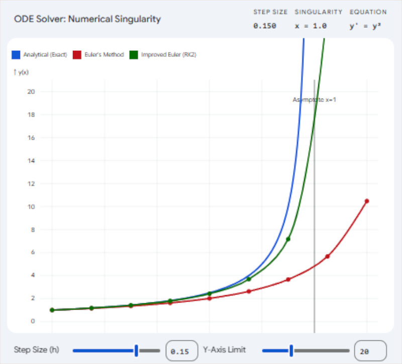
Gemini ODE Solver to see how Standard Euler and Improved Euler try (and ultimately fail) to track the true analytical curve as it approaches the vertical asymptote at x=1.

Implications for Numerical Methods

When dealing with ODEs that have singularities or highly erratic behavior within the interval of integration, standard fixed-step methods aren’t enough. Special care must be taken:

• Adaptive Step Size: Instead of a fixed $h$, modern solvers dynamically adjust the step size. They monitor the estimated error and automatically shrink $h$ as the solution approaches a singularity (taking tiny, careful steps), and widen it when the curve is flat and predictable.
• Alternative Methods: More sophisticated numerical solvers (like the widely used Runge-Kutta 4th Order, or RK45 which incorporates adaptive stepping) are required for complex, real-world differential equations.
• Analytical Insights: Never blindly trust a computer/algorithm! Understanding the underlying mathematical behavior of the ODE analytically will inform your choice of numerical method and help you interpret whether a “blow-up” in your data is a real physical phenomenon or just a failure of your algorithm.

To sum up, the Improved Euler's method offers a significant improvement in accuracy over the basic Euler's method by averaging the slopes at the beginning and end of each interval. However, it is important to be aware of potential pitfalls, such as singularities in the solution, which can render numerical methods quite ineffective without appropriate adjustments.

Bibliography

1. NPTEL-NOC IITM, Introduction to Galois Theory.
2. Algebra, Second Edition, by Michael Artin.
3. LibreTexts, Calculus and Calculus 3e (Apex). Abstract and Geometric Algebra, Abstract Algebra: Theory and Applications (Judson).
4. Field and Galois Theory, by Patrick Morandi. Springer.
5. Michael Penn, and MathMajor.
6. Contemporary Abstract Algebra, Joseph, A. Gallian.
7. YouTube’s Andrew Misseldine: Calculus. College Algebra and Abstract Algebra.
8. MIT OpenCourseWare [18.03 Differential Equations, Spring 2006], YouTube by MIT OpenCourseWare.
9. Calculus Early Transcendentals: Differential & Multi-Variable Calculus for Social Sciences.