Homogeneous Linear Systems with repeated real eigenvalues

Any fool can criticize, complain, and condemn —and most fools do. But it takes character and self-control to be understanding and forgiving, Dale Carnegie

Linear First-Order Systems: The Matrix Approach

A general linear first-order system of two variables has the form:

$\begin{cases} x' = a(t)x + b(t)y + r_1(t) \\\\ y' = c(t)x + d(t)y + r_2(t) \end{cases}$ where:

• $a(t), b(t), c(t)$, and $d(t)$ are functions of time $t$ (or constants in simpler cases).
• $r_1(t)$ and $r_2(t)$ represent external forcing functions or inputs.
• $x(t_0) = x_0$ and $y(t_0) = y_0$ are the initial conditions.

Homogeneous Linear Systems with Constant Coefficients

Let’s explore homogeneous linear systems of first-order ordinary differential equations (ODEs) with constant coefficients. Specifically, we will return to our egg-cooling temperature model:

$\begin{cases} x' = -2x + 2y \\\\ y' = 2x - 5y \end{cases}$ where:

• We have swapped $T_1$ and $T_2$ for standard variables $x$ and $y$ for simplicity.
• x(t) and y(t) are the dependent variables.
• t is the independent variable (typically representing time).
• x’ = $\frac{dx}{dt}$ and y’ = $\frac{dy}{dt}$ denote the first derivatives of x(t) and y(t) with respect to t.

The given system of ODE’s is a homogeneous linear system because:

• The equations are perfectly linear with respect to $x$ and $y$.
• There are no standalone forcing terms depending only on $t$.

There are no constant or forcing terms (i.e., terms that do not depend on x or y).

In a previous section, we solved this exact system using the substitution method (converting it into a single second-order ODE). Our solution was: $\begin{cases} x = C_1e^{-t} + C_2e^{-6t} \\\ y = \frac{1}{2}C_1e^{-t} - 2C_2e^{-6t} \end{cases}$

While substitution works for 2x2 systems, it becomes computationally messy (nightmarish) for larger systems. Instead, we will solve this using the Eigenvalue and Eigenvector method. This approach transforms the system into an algebraic problem, allowing us to find the general solution by identifying the system’s eigenvalues and corresponding eigenvectors.

Example: Repeated Real Eigenvalues (The Fish Tank Model)

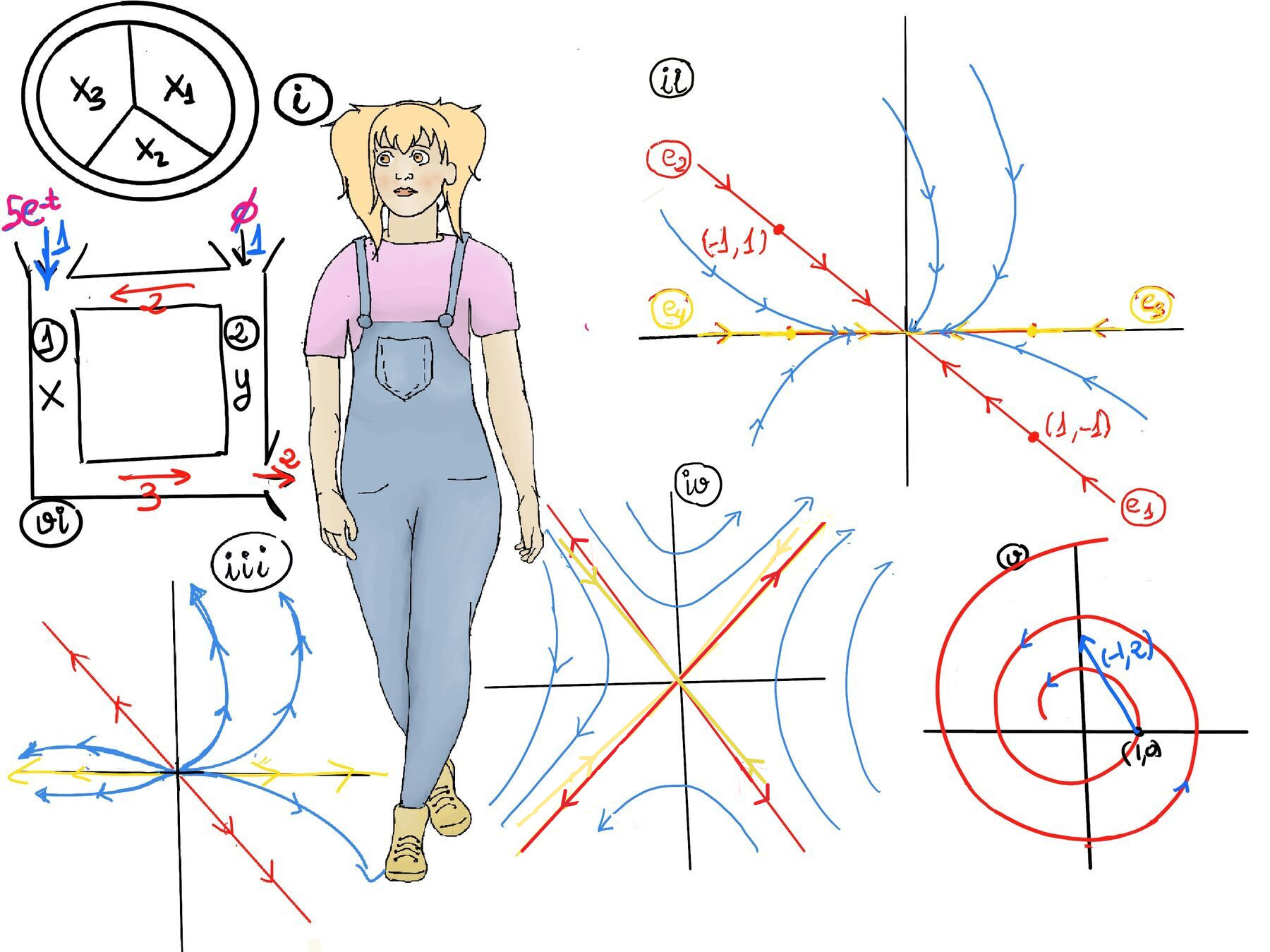
Consider a model where a fish tank is divided into three compartments, each maintained at different initial temperatures:

• $x_1(t)$ for the tropical region.
• $x_2(t)$ for the normal region.
• $x_3(t)$ for the ice region.

The compartments are perfectly insulated from the outside (external) environment, meaning no heat is lost or gained from outside the tank. Heat only flows between these compartments due to the temperature differences between them. Over time, these compartments exchange heat, and our goal is to determine how the temperatures in each compartment evolve over time (Refer to Figure i for a visual representation and aid in understanding it).

Step 0. Setting Up the Differential System

To represent this mathematically, let $x_i(t)$ represent the temperature in the i-th compartment at time t, where i = 1, 2, 3.

The heat flow from compartment i to compartment j is proportional to the difference in temperature between the compartments, following Newton’s Law of Cooling. That is, the rate at which heat flows is proportional to their temperature difference: $(x_j - x_i)$.

Let’s assume the proportionality constant for heat exchange between any two adjacent compartments is exactly $1$. The net rate of heat flow into compartment 1 is the sum of the heat flowing in from compartment 2 and compartment 3: $x_1' = 1 \cdot (x_2 - x_1) + 1 \cdot (x_3 - x_1) \implies[\text{Simplify, }] x_1' = -2x_1 + x_2 + x_3$

Because of the symmetry in our differential system (every compartment interacts with the other two equally), we obtain the following $3 \times 3$ system of ODEs:

$\begin{cases} x_1' = -2x_1 + x_2 + x_3 \\ x_2' = x_1 - 2x_2 + x_3 \\ x_3' = x_1 + x_2 - 2x_3 \end{cases}$

This system can be written in matrix form $X' = AX$ as:

$$\begin{pmatrix} x_1' \\ x_2' \\ x_3' \end{pmatrix} = \begin{pmatrix} -2 & 1 & 1 \\ 1 & -2 & 1 \\ 1 & 1 & -2 \end{pmatrix} \begin{pmatrix} x_1 \\ x_2 \\ x_3 \end{pmatrix}$$

Step 1: The Characteristic Equation

We now aim to find the general solution to this system, which requires solving for the eigenvalues and eigenvectors of the matrix A.

To find the eigenvalues, we solve the characteristic equation: |A - λI| = $\Bigl \vert\begin{smallmatrix}-2-λ & 1 & 1\\\ 1 & -2-λ & 1\\\ 1 & 1 & -2-λ\end{smallmatrix}\Bigr \vert =[\text{Expanding this 3×3 determinant yields a cubic polynomial:}] -(λ+2)^3-3(-2-λ)+2 = 0$

$−(8+12λ+6λ^2 +λ^3)−3(−2−λ)+2 = 0 ↭ (−8+6+2)+(−12λ+3λ)+(−6λ^2) −λ^3 =0 ↭\text{[Simplify and multiply both sides by -1]} λ^3 +6λ^2 +9λ = 0$

Factoring it: $λ(λ + 3)^2 = 0$.

The eigenvalues are:

• $\lambda_1 = 0$ (Single root)

• $\lambda_2 = \lambda_3 = -3$ (Repeated root with multiplicity 2)

• Step 2: Finding the Eigenvectors

For $\lambda_1 = 0$:

We solve $(A - 0I)\mathbf{v} = 0$:

$$\begin{pmatrix} -2 & 1 & 1 \\ 1 & -2 & 1 \\ 1 & 1 & -2 \end{pmatrix} \begin{pmatrix} a_1 \\ a_2 \\ a_3 \end{pmatrix} = \begin{pmatrix} 0 \\ 0 \\ 0 \end{pmatrix}$$

This leads to a dependent system where all rows sum to $0$.

• From row 2: $a_1 - 2a_2 + a_3 = 0 \implies a_3 = 2a_2 - a_1$.
• From row 1: $-2a_1 + a_2 + (2a_2 - a_1) = 0 \implies -3a_1 + 3a_2 = 0 \implies a_1 = a_2$.
• If $a_1 = a_2$, then $a_3 = 2(a_1) - a_1 = a_1$. Therefore, all components must be equal!

If we set $a_1 = 1$, we get the eigenvector: $\mathbf{v}_1 = \begin{pmatrix} 1 \\ 1 \\ 1 \end{pmatrix}$. Any scalar multiple of this vector is also an eigenvector.

Fundamental Solution 1: $X_1(t) = \begin{pmatrix} 1 \\ 1 \\ 1 \end{pmatrix}e^{0t} = \begin{pmatrix} 1 \\ 1 \\ 1 \end{pmatrix}$

💡 Physical Intuition: This constant solution represents the state where all three compartments share the exact same temperature. Because there is no temperature difference, no heat flows, and the derivatives are all exactly $0$.

For $\lambda_{2,3} = -3$ (The Repeated Root):

We solve $(A - (-3)I)\mathbf{v} = 0 \implies (A + 3I)\mathbf{v} = 0$:

$$\begin{pmatrix} 1 & 1 & 1 \\ 1 & 1 & 1 \\ 1 & 1 & 1 \end{pmatrix} \begin{pmatrix} a_1 \\ a_2 \\ a_3 \end{pmatrix} = \begin{pmatrix} 0 \\ 0 \\ 0 \end{pmatrix}$$

This system collapses into a single, perfectly identical equation repeated three times: $a_1 + a_2 + a_3 = 0$

This single equation defines a 2-dimensional plane in $\mathbb{R}^3$. To capture the full space, we need to find two linearly independent vectors that satisfy this equation.

• If we choose $a_1 = 1, a_2 = 0$, then $a_3 = -1$. This gives $\mathbf{v}_2 = \begin{pmatrix} 1 \\ 0 \\ -1 \end{pmatrix}$.
• If we choose $a_1 = 1, a_2 = -1$, then $a_3 = 0$. This gives $\mathbf{v}_3 = \begin{pmatrix} 1 \\ -1 \\ 0 \end{pmatrix}$.
• The reader should be cautious. A vector like $(0, 1, -1)^T$ also satisfies the equation, but it is just a linear combination of our first two vectors: $\mathbf{v}_2 - \mathbf{v}_3$. We strictly only need two independent basis vectors.

Fundamental Solutions 2 & 3: $X_2(t) = \begin{pmatrix} 1 \\ 0 \\ -1 \end{pmatrix}e^{-3t}$ and $X_3(t) = \begin{pmatrix} 1 \\ -1 \\ 0 \end{pmatrix}e^{-3t}$

Step 3: General Solution and Long-Term Behavior

The general solution is the linear combination of our three fundamental solutions: $\boxed{X(t) = C_1 \begin{pmatrix} 1 \\ 0 \\ -1 \end{pmatrix}e^{-3t} + C_2 \begin{pmatrix} 1 \\ -1 \\ 0 \end{pmatrix}e^{-3t} + C_3 \begin{pmatrix} 1 \\ 1 \\ 1 \end{pmatrix}}$

Long-Term Behavior ($t \to \infty$):

As time progresses to infinity, the exponential term $e^{-3t}$ shrinks to $0$. Therefore, the entire dynamic part of the system decays away, and the solution approaches a constant state: $X(t) \to C_3 \begin{pmatrix} 1 \\ 1 \\ 1 \end{pmatrix}$

This perfectly matches the physics! The temperatures will equalize over time. All compartments tend toward the exact same final temperature ($C_3$), reaching total thermal equilibrium ( corresponding to the eigenvalue $\lambda = 0$).

Understanding Repeated Eigenvalues

In this fish tank example, we encountered a repeated eigenvalue ($\lambda = -3$) which appeared twice as a root of the characteristic polynomial.

To formalize how we handle this, we define two types of multiplicity:

1. Algebraic Multiplicity ($m$): The number of times the eigenvalue appears as a root in the characteristic equation. For $\lambda = -3$, $m=2$.
2. Geometric Multiplicity ($g$): The number of linearly independent eigenvectors we can actually find for that eigenvalue (i.e., the dimension of the null space of $A - \lambda I$).

An eigenvalue is considered Complete (or non-defective) if its geometric multiplicity exactly matches its algebraic multiplicity ($g = m$). This means we have enough linearly independent eigenvectors to form a complete basis for the solution. In our fish tank problem, $\lambda = -3$ had an algebraic multiplicity of $2$, and we successfully found $2$ independent eigenvectors for it. It was a complete eigenvalue, so finding the solution was straightforward.

An eigenvalue is considered Defective if we cannot find enough independent eigenvectors to match its algebraic multiplicity ($g < m$). If an eigenvalue is defective, the matrix $A$ is not diagonalizable, and our standard $X(t) = \mathbf{v} e^{\lambda t}$ method will “run out” of vectors, preventing us from building the full general solution. To solve ODE systems with defective eigenvalues, we have to use a special technique called Generalized Eigenvectors (which involves multiplying terms by $t$ to regain linear independence).

The Spectral or Principal Axis Theorem

The Spectral or Principal Axis Theorem is a fundamental result in linear algebra with significant and profound implications in various fields such as physics, engineering, and applied mathematics. It essentially guarantees that certain complex matrices can be broken down into a much simpler, highly structured form.

The theorem states that for any real symmetric matrix, the eigenvalues are real, and there exists an orthogonal basis of eigenvectors of the matrix.

Specifically, if $A$ is a real n × n symmetric matrix (where $A = A^T$), then:

• Real Eigenvalues: All eigenvalues of the matrix A are real numbers. This means that when we solve the characteristic equation $\det(A - \lambda I) = 0$, every solution $\lambda$ (the eigenvalues) will reside strictly on the real number line —no imaginary or complex components will appear.

• Complete, Orthogonal Eigenvalues: All eigenvalues are complete, meaning that for the matrix A, there exists a full set of n linearly independent eigenvectors that are mutually orthogonal.

Because there is a corresponding eigenvector for each eigenvalue, the collection of all such eigenvectors forms a complete basis for $\mathbb{R}^n$. Since these eigenvectors can be chosen to be perfectly orthogonal (at right angles to one another), we can use an orthogonal transformation to simplify the matrix $A$ into a purely diagonal form. This effectively “uncouples” interacting variables in a system, making complex calculations drastically simpler.

Bibliography

1. NPTEL-NOC IITM, Introduction to Galois Theory.
2. Algebra, Second Edition, by Michael Artin.
3. LibreTexts, Calculus and Calculus 3e (Apex). Abstract and Geometric Algebra, Abstract Algebra: Theory and Applications (Judson).
4. Field and Galois Theory, by Patrick Morandi. Springer.
5. Michael Penn, and MathMajor.
6. Contemporary Abstract Algebra, Joseph, A. Gallian.
7. YouTube’s Andrew Misseldine: Calculus. College Algebra and Abstract Algebra.
8. MIT OpenCourseWare [18.03 Differential Equations, Spring 2006], YouTube by MIT OpenCourseWare.
9. Calculus Early Transcendentals: Differential & Multi-Variable Calculus for Social Sciences.