Homogeneous First-Order ODE's

When you have eliminated the impossible, whatever remains, however improbable, must be the truth, Sherlock Holmes.

Recall. Algebraic and differential equations.

An algebraic equation is a mathematical statement asserting that two algebraic expressions are equal.. These expressions are constructed using:

1. Dependent and independent variables. Variables are symbols representing unknown quantities. Variables can be:
   Independent Variables: Variables or input that can be chosen (or change) freely.
   Dependent Variables: Variables that depend on the independent variables.
2. Constants. Fixed numerical values that do not change, e.g., 2, π, 7.
3. Algebraic operations. Operations such as addition, subtraction, multiplication, division, exponentiation, powers, and root.

An algebraic equation typically has the following general form: Expression₁ = Expression₂, where the two expressions are set equal to each other.

Examples: y = 2x + 4 (simple linear equation, represents a straight line with a slope of 2 and a y-intercept of 4), ax² + bx + c = 0 (quadratic equation, it represents a parabola), $ln(xy + t) = z·sin(\sqrt{x})$.

Definition. A differential equation is an equation that involves one or more functions and their derivatives. It relates the function itself (the dependent variable), its derivatives with respect to one or more independent variables (rates of change), and the independent variable(s) themselves, e.g., $\frac{dy}{dx} = 3x +5y, y' + y = 4xcos(2x), \frac{dy}{dx} = x^2y+y, etc.$

If an algebraic equation is a “snapshot” of a relationship, a differential equation is the “instruction manual” for how that relationship moves and changes.

Key Components (e.g., $\frac{dy}{dx} = 3x +5y$):

• Dependent variables: The function y (or y(x)) we are trying to find or solve for. Variable(s) (y) that depend on one or more other variables.
• Independent variables: Variable(s) (x) upon which the dependent variables depend and we differentiate with respect to (often time or space).
• Derivatives: Expressions like $\frac{dy}{dx}$ or y’ that represent the rate at which the dependent variable (y) change with respect to the independent variable (x).

Existence and Uniqueness Theorem

The Existence and Uniqueness Theorem provides crucial insight into the behavior of solutions to first-order differential equations ODEs. It answers two fundamental questions: Is there a solution? and Is it the only one? It states that if:

• The function $f(x, y)$ (the right-hand side of the ODE when written as $y' = f(x, y)$) is continuous in some neighborhood around a specific point $(x_0, y_0)$ and
• Its partial derivative with respect to y, denoted as $\frac{\partial f}{\partial y}$, is also continuous near $(x_0, y_0)$.

Then, the differential equation y' = f(x, y) has a unique solution to the initial value problem through the point (x₀, y₀), meaning that it perfectly satisfies the initial condition $y(x_0) = y_0$.

This theorem is a mathematician’s safety net: it ensures that under these well-behaved conditions, a solution definitively exists and is absolutely unique near $x = x_0$. The physical system modeled by the ODE will only follow one distinct path.

Homogeneous First-Order ODE’s

Definition. A homogenous first-order ODE is a differential equation where the right-hand side can be expressed as a function of the ratio $\frac{y}{x}$. The general form is $y' = \frac{dy}{dx} = F(\frac{y}{x})$.

This form implies that the equation is scale-invariant. This means that if both variables x and y are scaled by the same non-zero constant, the fundamental form of the equation remains completely unchanged. This unique property makes homogeneous ODEs perfectly suited for specific substitution methods that easily untangle and simplify their solutions.

Scaling Invariance (Zoom Symmetry)

To prove this property, let us rescale both x and y by the same factor a, such that $x = ax_1$ and $y = ay_1$, where a is a non-zero constant (a ≠ 0).

First, we calculate the differentials: $dx = a dx_1, dy = a dy_1$.

Now, substitute these into the derivative $\frac{dy}{dx}$: $\frac{dy}{dx} = F(\frac{y}{x}) ↭ \frac{ady_1}{adx_1} = \frac{dy_1}{dx_1} = F(\frac{y}{x}) = F(\frac{ay_1}{ax_1}) = F(\frac{y_1}{x_1}) ↭[\text{ the scaled version of the equation becomes:}] \frac{dy_1}{dx_1} = F(\frac{y_1}{x_1})$

This shows that the form of the equation remains exactly the same after scaling, making the equation invariant under zoom. In simple terms, zooming in or out on the graph of the solution (scaling both axes equally) does not change the underlying differential equation or the geometry of its slope field.

Examples of Homogeneous ODEs

Here is how we can algebraically verify if an equation is homogeneous:

• Example 1. Consider the equation $y' = \frac{x^2y}{x^3+y^3}$.

To check if it is homogeneous, we divide both numerator and denominator by $x^3$: $y' = \frac{\frac{y}{x}}{1+(\frac{y}{x})^3}$ The right-hand side of the equation is now exclusively a function of $\frac{y}{x}$, confirming that the ODE is indeed homogeneous.

• Example 2. Consider the differential equation $x\frac{dy}{dx} = y + 2\sqrt{xy}$.

To check if it is homogeneous, we divide all terms by x: $\frac{dy}{dx} = \frac{y}{x} + \frac{2\sqrt{xy}}{x}$

Assume that x is positive, then we can rewrite the denominator x as $\sqrt{x^2}=|x| = x$: $\frac{dy}{dx} = \frac{y}{x} + \frac{2\sqrt{xy}}{\sqrt{x^2}} ↭ \frac{dy}{dx} = \frac{y}{x} + 2\sqrt{\frac{y}{x}}$. Again, the right-hand side of the equation is now a function of $\frac{y}{x}$, confirming that the ODE is homogeneous.

• Example 3. Consider a second equation $xy' = \sqrt{x^2 + y^2}$

Divide both sides by x (and bring it inside the square root as $x^2$) gives, $y' = \sqrt{1+(\frac{y}{x})^2}$. Again, the right-hand side depends solely on $\frac{y}{x}$, confirming homogeneity.

Solving Homogeneous ODEs

The core strategy for solving these equations relies on a clever substitution that takes advantage of the $\frac{y}{x}$ clustering.

1. Substitution. To solve an ODE of the form y’ = F($\frac{y}{x}$), the substitution z = $\frac{y}{x}$ is used, where z is a new variable representing the ratio $\frac{y}{x}$. This leverages the scale invariance to simplify the equation.

2. Differentiation. Consider y’ = F(y/x). If we define z = y/x, we can express y as y = zx. Differentiating both sides with respect to x requires the product rule: y’ = z’x + z where $z' = \frac{dz}{dx}$.

3. Substituting back into the original ODE y’ = F(y/x), we get: z’x + z = F(z) ↭[This can be rearranged as:] $x\frac{dz}{dx} = F(z)-z$. This equation is separable.

4. Separate variables. Move all z terms to one side and x terms to the other: $\frac{dz}{F(z)-z} = \frac{dx}{x}$.

5. Integrate both sides. $\int \frac{dz}{F(z)-z} = \int \frac{dx}{x}$. Solve the integrals to find z as a function of x, considering any necessary techniques (e.g., partial fractions, substitution).

6. Back-Substitution. Once z(x) is found, substitute back z = $\frac{y}{x}$ to compute y(x).

7. Apply initial conditions. If provided, plug in your given coordinates to solve for the constant of integration and find the particular solution.

Exercises Homogeneous ODEs

• Solve the differential equation $(xy+y^2+x^2)dx -x^2dy = 0$

1. Rewrite the Equation. First, rearrange to isolate the differential terms: $(xy+y^2+x^2)dx -x^2dy = 0↭ x^2dy = (xy +y^2+x^2)dx$. Divide both sides by x²dx, assuming x ≠ 0: $\frac{dy}{dx} = \frac{y}{x} + (\frac{y}{x})^2 + 1$ This confirms that the ODE is homogeneous.

2. Substitution, z = $\frac{y}{x}$. This substitution leverages the scale-invariance property of homogeneous first-order ODEs.

3. Differentiation. y = zx ⇒[By the chain rule] y’ = z’x + z where $z' = \frac{dz}{dx}$.

4. Substituting back into the original ODE. y’ = F(y/x), we get: $z'x + z = z + z^2 +1$
   This can be rearranged and simplified (the z terms on both sides cancel out) as: $x\frac{dz}{dx} = z^2 +1$.
   This equation is separable.

5. Separate variables: $\frac{dz}{z^2+1} = \frac{dx}{x}$.

6. Integrate both sides. $\int \frac{dz}{z^2+1} = \int \frac{dx}{x}↭ tan^{-1}(z) = ln|x| + C$ \begin{matrix} Take the tangent of both sides to isolate z: $tan(tan^{-1}(z)) = tan(ln|x| + C) \iff z = tan(ln|x| + C)$.

7. Back-Substitution. Once z(x) is found, substitute back z = $\frac{y}{x}$ to compute y(x). $\frac{y}{x} = tan(ln|x| + C)$.

Therefore, the general solution to the differential equation is: $\boxed{y = x·tan(ln|x| + C)}$.

• Solve $2xy\frac{dy}{dx} = x^2+2y^2$

1. Identify and Rewrite the Equation. First, we isolate the derivative $\frac{dy}{dx}$ (or $y'$) to check the structure of the equation: $2xy\frac{dy}{dx} = x^2+2y^2 ↭ \frac{dy}{dx} = \frac{x^2+2y^2}{2xy} ↭ \frac{dy}{dx} = \frac{x}{2y}+\frac{y}{x} ↭ \frac{dy}{dx} = \frac{1}{2}·(\frac{y}{x})^{-1} + \frac{y}{x}$. The right-hand side of the equation is now expressed entirely in terms of $\frac{y}{x}$, confirming that the differential equation is homogeneous.
2. Introduce the Substitution. For homogeneous equations, we use the substitution: z = $\frac{y}{x}$ where $z$ is a function of $x$.
3. Differentiate the Substitution. Using the Product Rule to differentiate $y = zx$ with respect to $x$, we get: $\frac{dy}{dx} = z + x\frac{dz}{dx}$.
4. Substituting back into the Original Equation. Replace $\frac{dy}{dx}$ with $(z + x\frac{dz}{dx})$ and $\frac{y}{x}$ with $z$ in the equation from Step 1: $z'x + z = \frac{1}{2}z^{-1}+z$ ↭[This can be simplified and rearranged as:] $x\frac{dz}{dx} = \frac{1}{2z}$. This equation is separable.
5. Separate Variables. Now that the equation is simplified, we move all $z$ terms to one side and all $x$ terms to the other: $zdz = \frac{dx}{2x}$.
6. Integrate both sides. Integrate to find the relationship between $z$ and $x$: $\int zdz = \int \frac{dx}{2x}↭ \frac{z^2}{2} = \frac{1}{2}ln|x|+C↭[\text{Multiply by 2}] z^2 = ln|x|+ C'$. Consider that C′ = 2C, but for simplicity, we’ll still denote it as C.
7. Back-Substitution. Once z(x) is found, substitute back z = $\frac{y}{x}$ to compute y(x). $(\frac{y}{x})^2 = ln|x|+ C ↭ \frac{y^2}{x^2} = ln|x| + C ↭ y^2 = x^2(ln|x| + C)$.
8. Solve for y. Taking the square root of both sides gives the explicit general solution: $\boxed{y = \pm x\sqrt{\ln|x| + C}}$

Notes

• The solution is defined where $\ln|x| + C \ge 0$.
• The substitution $z = \frac{y}{x}$ requires $x \neq 0$.
• The ± is essential when solving from $y^2 = \dots$; it should not be absorbed into the constant.

The Path of a Boat Under a Lighthouse Beam

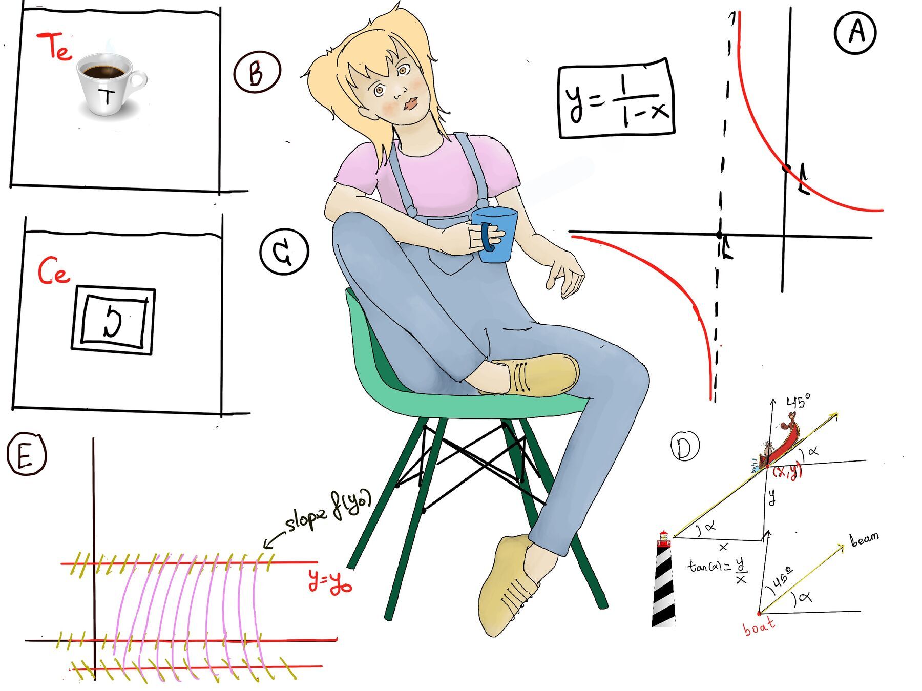
A lighthouse tracks a hostile boat (this is not just a boat; it’s a floating fortress of illicit activity, where trust is scarce and betrayal lurks just beneath the surface) moving at a constant angle 45° to the light beam. The lighthouse adjusts its beam to keep the boat illuminated. We aim to determine the boat’s path y = y(x).

Modeling the Boat’s Path

Let α be the angle between the boat’s position vector (the light beam) and the x-axis. From the geometry of the problem, we have: $\tan(\alpha) = \frac{y}{x}$ (Refer to Figure D for a visual representation and aid in understanding this setup).

Since the boat moves at an angle of 45° relative to the light beam, the slope of the boat’s path is: y’ = $\frac{dy}{dx}$ = tan(α + 45°). This is because the boat’s direction is offset by 45° from the line connecting it to the lighthouse.

Using the angle addition formula for tangent, tan(A + B) = $\frac{tan(A)+tan(B)}{1-tan(A)·tan(B)}$, and knowing that tan(45°) = 1, we can expand our slope equation: tan(α + 45°) = $\frac{tan(α)+tan(45)}{1-tan(α)·tan(45)} = \frac{tan(α)+1}{1-tan(α)}$

Substitute tan(α) = y/x into the expanded formula: $y'= \frac{\frac{y}{x}+1}{1-\frac{y}{x}}$. This equation is a homogeneous differential equation because the right-hand side is entirely a function of the ratio $\frac{y}{x}$.

Substitute Back into the ODE: To solve this, we introduce a new variable z = y/x, which means y = zx. Differentiating both sides with respect to x (using the product rule) yields: y’ = z’x + z.

Substituting into the ODE, we have: $z'x + z = \frac{z+1}{1-z} ↭[\text{Rearrange the equation}] x\frac{dz}{dx} = \frac{z+1}{1-z}-z = \frac{z+1}{1-z}-\frac{z(1-z)}{1-z}=\frac{z+1-z+z^2}{1-z} = \frac{1+z^2}{1-z} ↭ x\frac{dz}{dx} = \frac{1+z^2}{1-z}$

Separation of variables. Now, group all z terms on the left and x terms on the right: $\frac{1-z}{1+z^2}dz = \frac{dx}{x}$

Integrate both sides. $\int \frac{1-z}{1+z^2}dz = \int \frac{dx}{x}$

The left-hand side can be split into two standard integrals:

$\int \frac{1-z}{1+z^2}dz = \int \frac{1}{1+z^2}dz + \int \frac{-z}{1+z^2}dz = tan^{-1}(z)-\frac{1}{2}ln(1+z^2)$ because $\int \frac{z}{1+z^2}dz = \frac{1}{2}ln(1+z^2)$

Combined Integral Equation: $tan^{-1}(z)-\frac{1}{2}ln(1+z^2) = ln|x| + C ↭ tan^{-1}(z) = \frac{1}{2}ln(1+z^2) + ln|x| + C ↭tan^{-1}(z) = ln(\sqrt{1+z^2}) + ln|x| + C$.

Using the logarithm power rule, we can rewrite the 1/x multiplier as a square root inside the natural log.

Back-Substitution. Substitute z = y/x back into the equation: $tan^{-1}(\frac{y}{x}) = ln(\sqrt{1+(\frac{y}{x})^2})+ln(x) + C = ln(\frac{\sqrt{x^2+y^2}}{|x|})+ln|x| + C$

Recall the logarithm quotient rule ln(a/b) = ln(a)-ln(b): $tan^{-1}(\frac{y}{x}) = ln(\sqrt{(x^2+y^2)})-ln|x|+ln|x|+C ↭[\text{The ln|x| terms brilliantly cancel each other out, leaving:}] tan^{-1}(\frac{y}{x}) = ln(\sqrt{x^2+y^2}) + c$

Converting to Polar Coordinates. To make sense of this path, we convert it to polar coordinates, where r is the radial distance and θ is the angle, with $r=\sqrt{x^2+y^2}, θ = tan^{-1}(\frac{y}{x})$, so our equation becomes $θ = ln(r)+C$.

To solve for r, isolate the natural log and exponentiate both sides: $ln(r) = \theta - C \implies r = e^{\theta -C} = e^{-C}\cdot e^{\theta}$. Since $e^{-C}$ is just another constant, let’s call it $C_1$, $r = C_1e^{\theta}$.

Thus, the boat’s path is described by the equation $\boxed{r = C_1e^θ}$, which is the equation of an exponential spiral. It is a type of spiral curve that grows outward as it revolves around a central point. The defining characteristic is that the distance from the center increases exponentially as the angle increases.

An exponential spiral, also known as a logarithmic spiral, is a common curve that frequently appears in nature, such as in the shells of mollusks, the arms of hurricanes, and the swirl of galaxies. In this context, it perfectly models the path of our hostile boat moving away from a lighthouse while stubbornly maintaining a constant 45° angle with the beam.

• The constant angle between the boat’s path and the beam dictates (or results into) the exponential relationship between r and θ.
• The exponential spiral reflects how the boat escapes, increasing its distance (r) exponentially relative to the sweeping angle of the lighthouse beam.

Bibliography

1. NPTEL-NOC IITM, Introduction to Galois Theory.
2. Algebra, Second Edition, by Michael Artin.
3. LibreTexts, Calculus and Calculus 3e (Apex). Abstract and Geometric Algebra, Abstract Algebra: Theory and Applications (Judson).
4. Field and Galois Theory, by Patrick Morandi. Springer.
5. Michael Penn, and MathMajor.
6. Contemporary Abstract Algebra, Joseph, A. Gallian.
7. YouTube’s Andrew Misseldine: Calculus. College Algebra and Abstract Algebra.
8. MIT OpenCourseWare [18.03 Differential Equations, Spring 2006], YouTube by MIT OpenCourseWare.
9. Calculus Early Transcendentals: Differential & Multi-Variable Calculus for Social Sciences.