Fourier Series. Square-Wave, Gibbs Phenomenon, & Uniqueness

If you’re going through hell, keep on going, Winston Churchill.

Introduction to Fourier Series

In this section, we introduce the concept of the Fourier series, a powerful mathematical tool used to represent virtually any periodic function as an infinite sum of simple sine and cosine waves.

This technique is incredibly useful when analyzing physical systems modeled by inhomogeneous second-order linear differential equations of the form: $y'' + ay' + by = f(t)$ where:

• $y(t)$ is the unknown response or behavior of the system (what we want to solve for).
• $f(t)$ is the known forcing function representing an external, periodic push or pull on the system.
• $a$ and $b$ are constants that describe inherent physical characteristics of the system, such as damping (friction) or stiffness (spring constant).

A Fourier series allows to write or express any periodic function f(t) (with a period of $2\pi$) as an infinite sum of trigonometric functions. The general form of a Fourier series is given by: $\boxed{f(t) = \frac{a_0}{2} + \sum_{n=1}^\infty [a_ncos(nt)+b_nsin(nt)]}$ where:

• $\frac{a_0}{2}$ is the constant term, representing the average (or “DC”) value of the function over one full period. It shifts the entire wave up or down on the y-axis.
• $a_n$ and $b_n$ (The Fourier Coefficients): These constants represent the amplitudes of the respective cosine and sine terms. They dictate “how much” of each specific wave is needed to build the original function.
• $n$ (The Harmonic Number): This is a positive integer ($1, 2, 3, ...$) that determines the frequency of each term. $n=1$ is the fundamental frequency, $n=2$ is the second harmonic (twice as fast), $n=3$ is the third harmonic, and so on.

If $f(t)$ is periodic with period $2\pi$, its Fourier series is: $f(t) = \frac{a_0}{2} + \sum_{n=1}^\infty \left[ a_n\cos(nt) + b_n\sin(nt) \right]$ where the coefficients are given by Euler’s formulas:

$\boxed{a_0 = \frac{1}{\pi}\int_{-\pi}^{\pi} f(t)dt}, \boxed{a_n = \frac{1}{\pi}\int_{-\pi}^{\pi} f(t)\cos(nt)dt}, \text{ and } \boxed{b_n = \frac{1}{\pi}\int_{-\pi}^{\pi} f(t)\sin(nt)dt}$

Example: Fourier Series of the Square-Wave Function

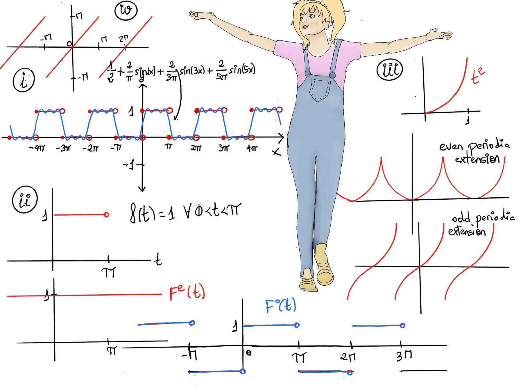
The square-wave function is a classic example used to demonstrate the remarkable power of Fourier series in representing periodic functions, even those with discontinuities. It shows us how a continuous mathematical tool (trigonometry) can perfectly describe a discontinuous physical reality (a signal switching instantly on and off).

This specific square-wave oscillates between two levels, $0$ and $1$, over one period $[-\pi, \pi]$. Formally, the function $f(t)$ is defined as:

This function is periodic with a period of $2\pi$, meaning $f(t+2\pi) = f(t)$ for all $t$.

Since it is periodic, it has a Fourier series representation of the form: $f(t) = \frac{a_0}{2} + \sum_{n=1}^\infty \left[ a_n\cos(nt) + b_n\sin(nt) \right]$

Our task is to compute the Fourier coefficients ($a_0$, $a_n$, and $b_n$) and express the function as a Fourier series.

Step 1: The Constant Term ($a_0$)

The $a_0$ term represents the average value (or “DC offset”) of the function over one full period.

$a_0 = \frac{1}{\pi}\int_{-\pi}^{\pi} f(t)dt$

Since $f(t) = 0$ for the left half of the period ($-\pi \le t < 0$) and $f(t) = 1$ for the right half ($0 \le t < \pi$), the integral simplifies to just the right half: $a_0 = \frac{1}{\pi}\int_{0}^{\pi} 1 dt = \frac{1}{\pi} \left[ t \right]_{0}^{\pi} = \frac{1}{\pi}(\pi - 0) = 1$

Thus, the constant term in the Fourier series is: $\frac{a_0}{2} = \frac{1}{2}$

This makes intuitive sense: if a signal spends half its time at $0$ and half its time at $1$, its average value is $0.5$.

Step 2: The Cosine Coefficients ($a_n$)

Next, we calculate the coefficients for the cosine terms. $a_n = \frac{1}{\pi}\int_{-\pi}^{\pi} f(t)\cos(nt)dt = \frac{1}{\pi}\int_{0}^{\pi} \cos(nt)dt$

Integrating the cosine function yields a sine function: $a_n = \frac{1}{n\pi}\sin(nt)\bigg|_{0}^{\pi} = \frac{1}{n\pi}[\sin(n\pi) - \sin(0)]$

Because $\sin(n\pi) = 0$ for all integers $n$, and $\sin(0) = 0$: $a_n = \frac{1}{n\pi}[0 - 0] = 0$

Why did this happen? The absence of cosine terms occurs because of symmetry. If you take our square wave and subtract its average value of $\frac{1}{2}$, it becomes an odd function (symmetric about the origin, jumping between $-0.5$ and $0.5$). Cosine is an even function. An odd function can only be constructed using other odd functions (like sine waves).

Step 3: The Sine Coefficients ($b_n$)

Now, we calculate the coefficients for the sine terms. $b_n = \frac{1}{\pi}\int_{-\pi}^{\pi} f(t)\sin(nt)dt = \frac{1}{\pi}\int_{0}^{\pi} \sin(nt)dt$

Integrating the sine function yields a negative cosine function: $b_n = \frac{-1}{n\pi}\cos(nt)\bigg|_{0}^{\pi} = \frac{-1}{n\pi}(\cos(n\pi) - \cos(0))$

Recall the highly useful trigonometric identity that $\cos(n\pi) = (-1)^n$, and also $\cos(0) = 1$. Substituting these into our expression, we get: $b_n = \frac{-1}{n\pi}\left((-1)^n - 1\right)$

This creates an alternating behavior depending on whether $n$ is even or odd:

• If $n$ is even (e.g., 2, 4, 6): $(-1)^n = 1$. The term inside the parenthesis becomes $(1 - 1) = 0$. So, $b_n = 0$.
• If $n$ is odd (e.g., 1, 3, 5): $(-1)^n = -1$. The term inside the parenthesis becomes $(-1 - 1) = -2$.

Therefore, for odd $n$ (which we can write as $n = 2k - 1$ for $k = 1, 2, 3 \cdots$): $b_n = \frac{-1}{n\pi}(-2) = \frac{2}{n\pi}$

Step 4: Constructing the Final Fourier Series

Now that we have all our coefficients ($a_0 = 1$, $a_n = 0$, $b_{\text{even}} = 0$, $b_{\text{odd}} = \frac{2}{n\pi}$), we can assemble the final series.

$f(t) = \frac{1}{2} + \sum_{k=1}^\infty \frac{2}{(2k-1)\pi}\sin((2k-1)t)$

Expanding the first few terms of this infinite sum gives us: $f(t) = \frac{1}{2} + \frac{2}{\pi}\sin(t) + \frac{2}{3\pi}\sin(3t) + \frac{2}{5\pi}\sin(5t) + \dots$

Factoring out the common $\frac{2}{\pi}$ provides the cleanest representation. The final Fourier Series for the Square-Wave is as follows: $\boxed{f(t) = \frac{1}{2} + \frac{2}{\pi}\left[ \sin(t) + \frac{1}{3}\sin(3t) + \frac{1}{5}\sin(5t) + \dots \right]}$

Discontinuities and the Gibbs Phenomenon

The underlying square wave (in one standard convention) is: $f(t) = \begin{cases} 0, & -\pi \le t < 0 \\ 1, & 0 \le t < \pi \end{cases}$, and then extended periodically with period $2\pi$. So the discontinuities happen at all points where the periodic extension “glues” these pieces together: $t = k\pi$ (where $k$ is any integer).

A fundamental theorem of Fourier analysis states: At any discontinuity $t_0$, the Fourier series converges to the average of the left and right limits. For the square wave:

• Left limit a the jump: $f(t_0^{-}) = 0$.
• Left limit a the jump: $f(t_0^{+}) = 1$.
• So the Fourier series converges to: $\frac{0+1}{2}=\frac{1}{2}$

In conclusion, this Fourier series is completely valid for all $t$ except at the exact moments of discontinuity, which occur at $t = k\pi$ (where $k$ is any integer). At these vertical jump points, the Fourier series converges to exactly $\frac{1}{2}$ (the midpoint of the jump).

Adding more terms (higher harmonics) to the Fourier series improves the approximation of the square-wave function, creating steeper, sharper walls. However, this reveals a fascinating mathematical quirk known as the Gibbs Phenomenon.

Because we are trying to approximate an instantaneous, non-differentiable jump using smooth, perfectly differentiable sine waves, the sine waves will always overshoot the top and bottom corners of the square wave by about 9%. Even if you add a million terms to the series, this overshoot never goes away; it just gets squished closer and closer to the wall of the jump!

The Uniqueness of Fourier Series

The uniqueness theorem is often glossed over, but it is the absolute bedrock of spectral analysis and signal processing. Without it, we could not trust that a frequency spectrum uniquely identifies a specific wave!

A fundamental property of the Fourier series is its uniqueness, which ensures that each periodic function corresponds to one, and only one, specific set of Fourier coefficients. In other words, the Fourier series provides an unique way to represent a periodic function as an infinite sum of sine and cosine functions.

Theorem (Uniqueness of Fourier Series): If two functions $f(t)$ and $g(t)$ are periodic with period $2L$ (or $2\pi$), and they are equal almost everywhere on the interval $[-L, L]$, then their Fourier series representations are mathematically identical.

This means that the Fourier coefficients $a_n$ and $b_n$ calculated for $f(t)$ will perfectly match those calculated for $g(t)$: $a_n^{(f)} = \frac{1}{L}\int_{-L}^{L} f(t)\cos\left(\frac{n\pi t}{L}\right)dt = \frac{1}{L}\int_{-L}^{L} g(t)\cos\left(\frac{n\pi t}{L}\right)dt = a_n^{(g)}$, $b_n^{(f)} = \frac{1}{L}\int_{-L}^{L} f(t)\sin\left(\frac{n\pi t}{L}\right)dt = \frac{1}{L}\int_{-L}^{L} g(t)\sin\left(\frac{n\pi t}{L}\right)dt = b_n^{(g)}$

This result holds because the formulas used to compute the Fourier coefficients are derived from definite integrals. The integral measures the “area under the curve” over the interval $[-L, L]$. If $f(t)$ and $g(t)$ share the same area footprint, their integrals —and therefore their coefficients— must be absolutely equal.

Implications of Uniqueness

The uniqueness theorem guarantees that the mapping between a function’s time-domain shape and its frequency-domain spectrum is reliable.

• One-to-One Correspondence. A given periodic function corresponds to one and only one set of Fourier coefficients. This ensures the Fourier series serves as a unique “fingerprint” (or representation) for the function.
• Reliable Reconstruction: If you are given a set of Fourier coefficients, you can perfectly reconstruct the original function f(t) everywhere it is continuous.
• Handling Discontinuities: At points where the original function has a sudden jump (discontinuity), the reconstructed Fourier series will predictably converge to the exact midpoint (average) of that jump.

Conditions for the Existence of Fourier Coefficients

Fourier coefficients exist — and are unique — whenever the function is absolutely integrable on [-L, L], $\int_{-L}^{L} \lt \infty$. The Fourier series representation is unique up to equality almost everywhere.

The phrase “almost everywhere” is a formal mathematical term from measure theory, but its practical application is highly intuitive. If $f(t)$ is a smooth sine wave, and $g(t)$ is that exact same sine wave but with one single point shifted heavily upward, $f(t)$ and $g(t)$ will yield the exact same Fourier series. The integral simply ignores the infinitely thin anomaly!

Because Fourier coefficients are calculated using integrals (areas), changing the value of a function at a single isolated point —or even a finite number of isolated points— does not add or subtract any width. Since a point has zero width, it adds zero area to the integral. Thus:

• Changing finitely many points → no effect
• Changing countably many isolated points → still no effect
• Changing uncountably many points but on a set of measure zero → still no effect

To guarantee that the Fourier series corresponds to a unique function (up to measure-zero differences), we require:

• Piecewise Continuous: A function may have finitely many jump or removable discontinuities or finitely many corners, but cannot have infinitely many discontinuities accumulating inside the interval or undefined regions of positive measure. This ensures the function is well-behaved enough for the Fourier series to converge in the classical sense.
• Absolutely Integrable: The functions must be absolutely integrable over [-L, L], ensuring that the integrals used to compute the Fourier coefficients converge.
• Both functions are considered equal almost everywhere f(t) = g(t) for almost every t. This includes: ($\star$) finite number of differing points; ($\star$) countably many differing points; ($\star$) any measure-zero set.

Bibliography

1. NPTEL-NOC IITM, Introduction to Galois Theory.
2. Algebra, Second Edition, by Michael Artin.
3. LibreTexts, Calculus and Calculus 3e (Apex). Abstract and Geometric Algebra, Abstract Algebra: Theory and Applications (Judson).
4. Field and Galois Theory, by Patrick Morandi. Springer.
5. Michael Penn, and MathMajor.
6. Contemporary Abstract Algebra, Joseph, A. Gallian.
7. YouTube’s Andrew Misseldine: Calculus. College Algebra and Abstract Algebra.
8. MIT OpenCourseWare [18.03 Differential Equations, Spring 2006], YouTube by MIT OpenCourseWare.
9. Calculus Early Transcendentals: Differential & Multi-Variable Calculus for Social Sciences.