Fourier Series. Symmetry, Convergence, and Arbitrary Periods

Do not worry about your difficulties in mathematics. I can assure you mine are still greater, Albert Einstein

Introduction to Fourier Series

In this section, we introduce the concept of the Fourier series, a powerful mathematical tool used to represent virtually any periodic function as an infinite sum of simple sine and cosine waves.

This technique is incredibly useful when analyzing physical systems modeled by inhomogeneous second-order linear differential equations of the form: $y'' + ay' + by = f(t)$ where:

• $y(t)$ is the unknown response or behavior of the system (what we want to solve for).
• $f(t)$ is the known forcing function representing an external, periodic push or pull on the system.
• $a$ and $b$ are constants that describe inherent physical characteristics of the system, such as damping (friction) or stiffness (spring constant).

A Fourier series allows to write or express any periodic function f(t) (with a period of $2\pi$) as an infinite sum of trigonometric functions. The general form of a Fourier series is given by: $\boxed{f(t) = \frac{a_0}{2} + \sum_{n=1}^\infty [a_ncos(nt)+b_nsin(nt)]}$ where:

• $\frac{a_0}{2}$ is the constant term, representing the average (or “DC”) value of the function over one full period. It shifts the entire wave up or down on the y-axis.
• $a_n$ and $b_n$ (The Fourier Coefficients): These constants represent the amplitudes of the respective cosine and sine terms. They dictate “how much” of each specific wave is needed to build the original function.
• $n$ (The Harmonic Number): This is a positive integer ($1, 2, 3, ...$) that determines the frequency of each term. $n=1$ is the fundamental frequency, $n=2$ is the second harmonic (twice as fast), $n=3$ is the third harmonic, and so on.

If $f(t)$ is periodic with period $2\pi$, its Fourier series is: $f(t) = \frac{a_0}{2} + \sum_{n=1}^\infty \left[ a_n\cos(nt) + b_n\sin(nt) \right]$ where the coefficients are given by Euler’s formulas:

$\boxed{a_0 = \frac{1}{\pi}\int_{-\pi}^{\pi} f(t)dt}, \boxed{a_n = \frac{1}{\pi}\int_{-\pi}^{\pi} f(t)\cos(nt)dt}, \text{ and } \boxed{b_n = \frac{1}{\pi}\int_{-\pi}^{\pi} f(t)\sin(nt)dt}$

Even and Odd Functions

Before applying symmetry to Fourier series, we must rigorously define what makes a function “even” or “odd.”

Definition. A function $f(t)$ is called even if it acts like a mirror across the y-axis. Mathematically, it satisfies the condition: $f(-t) = f(t) \quad \text{for all }$, e.g., $t^2$, $\cos(t)$, $|t|$, $t^2 + 4$.

The graph is symmetric with respect to the y-axis. If you fold the graph paper in half along the y-axis, the left and right sides will perfectly align.

Definition. A function $f(t)$ is called odd if its negative side is the inverted version of its positive side. Mathematically, it satisfies the condition: $f(-t) = -f(t) \quad \text{for all } t$, e.g., $t^3$, $\sin(t)$, $2t^3 - 3t$.

The graph has rotational symmetry around the origin $(0,0)$. If you pin the graph at the origin and rotate it 180 degrees, it will look exactly the same.

The Multiplication Rules (Cheat Sheet)

When determining Fourier coefficients, we constantly multiply functions together. It is highly useful to memorize these rules, which work just like multiplying positive and negative numbers:

• Even $\times$ Even = Even
• Odd $\times$ Odd = Even
• Even $\times$ Odd = Odd

Fourier Series for Even and Odd Functions

The Fourier series for a general periodic function $f(t)$ with a period of $2\pi$ is: $f(t) = \frac{a_0}{2} + \sum_{n=1}^\infty \left[ a_n\cos(nt) + b_n\sin(nt) \right]$

Since cosine is an strictly even function and sine is a strictly odd function, the behavior of the Fourier coefficients ($a_n$ and $b_n$) depends heavily on the symmetry of $f(t)$. We can prove this using the Uniqueness Theorem.

Case 1: When $f(t)$ is an Even Function

If $f(t)$ is even, we know that $f(-t) = f(t)$. Let’s plug $-t$ into the general Fourier series: $f(-t) = \frac{a_0}{2} + \sum_{n=1}^\infty \left[ a_n\cos(-nt) + b_n\sin(-nt) \right]$

Because $\cos(-nt) = \cos(nt)$ and $\sin(-nt) = -\sin(nt)$, this becomes: $f(-t) = \frac{a_0}{2} + \sum_{n=1}^\infty \left[ a_n\cos(nt) - b_n\sin(nt) \right]$

Now, we set $f(-t)$ equal to the original $f(t)$ equation: $\frac{a_0}{2} + \sum_{n=1}^\infty \left[ a_n\cos(nt) - b_n\sin(nt) \right] = \frac{a_0}{2} + \sum_{n=1}^\infty \left[ a_n\cos(nt) + b_n\sin(nt) \right]$

By the Uniqueness of Fourier Series, the coefficients on both sides must match perfectly. The only way $-b_n$ can equal $+b_n$ is if $b_n = 0$.

Conclusion: The Fourier series for an even function contains only cosine terms (and possibly a constant $a_0$ term). All $b_n$ coefficients are zero.

Furthermore, because $f(t)$ is even and $\cos(nt)$ is even, their product $f(t)\cos(nt)$ is also even. Integrating an even function from $-\pi$ to $\pi$ is exactly double the area from $0$ to $\pi$. This drastically simplifies our calculations:

$\boxed{a_n = \frac{2}{\pi}\int_{0}^{\pi} f(t)\cos(nt)dt}$

Case 2: When $f(t)$ is an Odd Function

If $f(t)$ is odd, we know that $f(-t) = -f(t)$.

Evaluate f at −t: $f(-t) =\frac{a_0}{2} + \sum_{n=0}^\infty (a_ncos(n(-t))+b_nsin(n(-t)))$ =[cos(n(−t)) = cos(−nt) = cos(nt) (since cosine is even), sin(n(−t)) = sin(−nt) = −sin(nt) (since sine is odd).] $\frac{a_0}{2} + \sum_{n=0}^\infty (a_ncos(nt))-b_nsin(nt)$

Comparing with Original Fourier Series: $f(t) = \frac{a_0}{2} + \sum_{n=1}^\infty (a_ncos(nt)+b_nsin(nt))$

Multiply both sides of the original equation by −1: $-f(t) = -\frac{a_0}{2} + \sum_{n=0}^\infty (-a_ncos(nt)-b_nsin(nt))$

If a function f is odd f(-t) = -f(t), then by the Uniqueness of the Fourier Series we conclude that all the cosine terms must be zero, i.e., all $a_n$ and $a_0$ coefficients are zero.

Because $f(t)$ is odd and $\sin(nt)$ is odd, their product $f(t)\sin(nt)$ is even (Odd $\times$ Odd = Even). Therefore, we can use the same half-interval shortcut: $\boxed{b_n = \frac{2}{\pi}\int_{0}^{\pi} f(t)\sin(nt)dt}$

This simplification reduces computation and is valid because the integrand is symmetric about the origin.

Examples:

• f(t) = cos(t). Since cos(t) is an even function, its Fourier series contains only cosine terms. $a_n = \frac{2}{\pi}\int_0^\pi \cos(t)\cos(nt) dt$. This integral can be evaluated for each n.
  n = 1. $a_1 = \frac{2}{\pi}\int_0^\pi \cos(t)\cos(t) dt = \frac{2}{\pi}\cdot \frac{\pi}{2} = 1.$
  $n\neq 1$. Orthogonality gives: $\int_0^\pi \cos(t)\cos(nt)dt = 0$. So: $a_n = 0 \quad \text{for } n\neq 1.$
  Constant term, $a_0 = \frac{2}{\pi}\int_0^\pi \cos(t),dt = \frac{2}{\pi}[\sin t]_0^\pi = 0$.
  Final Fourier series: $\boxed{\cos t = \cos t}$. Not surprising — the function is already a single cosine mode.
• f(t) = sin(t). Since sin(t) is odd, its Fourier series contains only sine terms. $b_n=\frac{2}{π}\int_{0}^{π} \sin(t)\sin(nt)dt$.
  n = 1. $b_1 = \frac{2}{\pi}\int_0^\pi \sin(t)\sin(t) dt = \frac{2}{\pi}\cdot \frac{\pi}{2} = 1$
  $n\neq 1$. Orthogonality gives: $\int_0^\pi \sin(t)\sin(nt)dt = 0$. So: $b_n = 0 \quad \text{for } n\neq 1$.
  Final Fourier series: $\boxed{\sin t = \sin t} $. Again, the function is already a single sine mode.

Convergence of Fourier Series (Dirichlet’s Theorem)

Once we build a Fourier series, we need to know if it actually equals the function f(t) it was built from.

Theorem: If a function $f(t)$ is periodic (period $2\pi$) and satisfies Dirichlet’s conditions (piecewise continuous, finite number of extrema), then:

Bounded Extrema. The function must have a finite number of peaks (maxima) and valleys (minima) within the interval [−L,L]. It cannot oscillate infinitely fast (like the function $\sin(\frac{1}{t})$ near zero). In other words, the function cannot wiggle infinitely many times in a finite interval.

Let $S_N(t) = \frac{a_0}{2} + \sum_{n=1}^N \left[a_n\cos(nt) + b_n\sin(nt)\right]$ be its (N)-th partial Fourier sum.

1. At points of continuity. If $f(t)$ is continuous at a specific point $t_0$, the infinite Fourier series converges exactly to the true value of the function at that point: $\boxed{f(t_0) = \frac{a_0}{2} + \sum_{n=1}^\infty \left[ a_n\cos(nt_0) + b_n\sin(nt_0) \right]}$.
   $\boxed{\lim_{N\to\infty} S_N(t_0) = f(t_0)}$.
2. At jump discontinuities. If $f(t)$ has a “jump” discontinuity at $t_0$ (meaning it instantly snaps from one value to another), the Fourier series cannot mathematically occupy two places at once. Instead, it perfectly splits the difference. It converges to the exact midpoint (the average) of the left-hand limit $f(t_0^-)$ and the right-hand limit $f(t_0^+)$: $\text{Convergence at jump} = \frac{f(t_0^+) + f(t_0^-)}{2}$.
   $\lim_{N\to\infty} S_N(t_0) = \lim_{N \to ∞}[\frac{a_0}{2} + \sum_{n=1}^N (a_ncos(nt)+b_nsin(nt))] = \frac{f(t_0^+)+f(t_0^-)}{2}$
   Why the midpoint? Because the Fourier series is built from continuous basis functions (sines and cosines). A continuous sum cannot “jump,” so it lands at the only value that makes sense: the average of the two one-sided limits.

The Gibbs Phenomenon

While the series converges to the exact midpoint at the jump, it exhibits strange behavior immediately before and after the jump.

Because we are trying to force smooth, continuous sine waves to replicate a sharp, jagged cliff, the Fourier series will overshoot the top and bottom of the jump by about 9%. This oscillatory ringing is known as the Gibbs Phenomenon

Increasing the number of terms ($N$) in the Fourier series does not decrease the height of this 9% overshoot. It only compresses the width of the ringing, pushing the overshoot tighter and tighter against the wall of the discontinuity.

This behavior is one of the key reasons Fourier series are widely used to represent functions with jump discontinuities. Applications: modeling electrical signals (square waves, sawtooth waves); analyzing mechanical vibrations; solving partial differential equations (heat equation, wave equation).

Fourier Series Extension (Arbitrary Periods)

Up to this point, we have primarily dealt with functions that have a period of $2\pi$. However, in real-world applications, functions can have any arbitrary period. Let’s denote this arbitrary period as $2L$ (meaning the function repeats over the interval $[-L, L]$).

To apply our existing Fourier series knowledge, we need to mathematically stretch or compress our standard interval $[-\pi, \pi]$ to fit $[-L, L]$. We do this using a simple change of variables.

Let $t$ be our physical variable (where $t \in [-L, L]$), and let $u$ be our normalized angular variable (where $u \in [-\pi, \pi]$). The mapping between them is: $u = \frac{\pi}{L}t \quad \iff \quad t = \frac{L}{\pi}u$

By substituting this into our standard formulas, the Fourier series expansion for a function $f(t)$ with period $2L$ becomes: $\boxed{f(t) = \frac{a_0}{2} + \sum_{n=1}^\infty \left[ a_n\cos\left(\frac{n\pi}{L}t\right) + b_n\sin\left(\frac{n\pi}{L}t\right) \right]}$ where the generalized Fourier coefficients are defined as:

• $a_n = \frac{1}{L}\int_{-L}^{L} f(t)\cos\left(\frac{n\pi}{L}t\right)dt$
• $b_n = \frac{1}{L}\int_{-L}^{L} f(t)\sin\left(\frac{n\pi}{L}t\right)dt$

Symmetry Shortcuts for Period $2L$

Just like with the $2\pi$ period, symmetry can drastically reduce our workload:

• If $f(t)$ is even: $b_n = 0$. The series contains only cosine terms, and $a_n = \frac{2}{L}\int_{0}^{L} f(t)\cos\left(\frac{n\pi}{L}t\right)dt$.
• If $f(t)$ is odd: $a_n = 0$. The series contains only sine terms, and $b_n = \frac{2}{L}\int_{0}^{L} f(t)\sin\left(\frac{n\pi}{L}t\right)dt$.

Half-Range Expansions (Periodic Extensions)

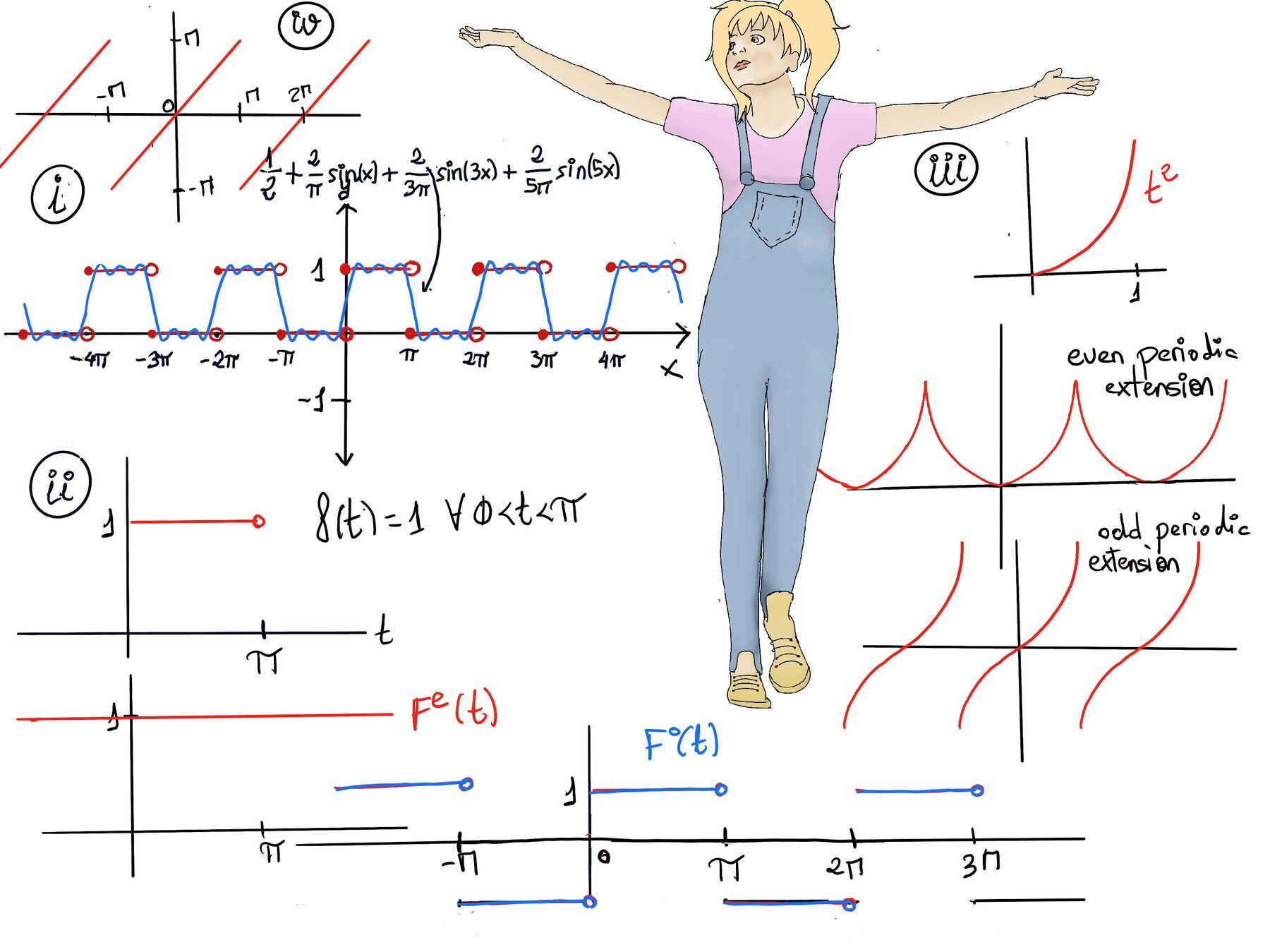
It is fairly common in engineering and physics for a function to be defined only on a finite, positive interval, such as $0 < t < L$. For example, you might be analyzing a plucked guitar string of length $L$.

Since the function does not exist outside of $(0, L)$, it doesn’t technically have a Fourier series yet. To use Fourier techniques, we must mathematically “invent” the rest of the function to make it periodic over the entire real line. We do this by creating a periodic extension. We have the freedom to choose how we draw the missing left half (from $-L$ to $0$). There are two highly useful (obviously distinct) ways to do this:

1. The Even Periodic Extension (Cosine Series).
   We define the even extension, $F^e(t)$, by mirroring the function across the y-axis.
   ($\star$) $F^e(t) = f(t)$ for $0 < t < L$ (Matches the original function).
   ($\star$) $F^e(-t) = f(t)$ for $-L < t < 0$ (Forces it to be even).
   ($\star$) $F^e(t)$ is periodic with period $2L$.
   Because $F^e(t)$ is mathematically forced to be an even function, its Fourier series will be a Half-Range Cosine Series.
2. The Odd Periodic Extension (Sine Series).
   We define the odd extension, $F^o(t)$, by rotating the function across the origin.
   $F^o(t) = f(t)$ for $0 < t < L$ (Matches the original function).
   $F^o(-t) = -f(t)$ for $-L < t < 0$ (Forces it to be odd).
   $F^o(t)$ is periodic with period $2L$.
   Because $F^o(t)$ is mathematically forced to be an odd function, its Fourier series will be a Half-Range Sine Series.

Key Idea 💡: Any function $f(t)$ defined only on $(0, L)$ can be represented perfectly well by either a pure cosine series or a pure sine series within that interval. The choice depends entirely on which extension you decide to build!

Bibliography

1. NPTEL-NOC IITM, Introduction to Galois Theory.
2. Algebra, Second Edition, by Michael Artin.
3. LibreTexts, Calculus and Calculus 3e (Apex). Abstract and Geometric Algebra, Abstract Algebra: Theory and Applications (Judson).
4. Field and Galois Theory, by Patrick Morandi. Springer.
5. Michael Penn, and MathMajor.
6. Contemporary Abstract Algebra, Joseph, A. Gallian.
7. YouTube’s Andrew Misseldine: Calculus. College Algebra and Abstract Algebra.
8. MIT OpenCourseWare [18.03 Differential Equations, Spring 2006], YouTube by MIT OpenCourseWare.
9. Calculus Early Transcendentals: Differential & Multi-Variable Calculus for Social Sciences.