Finding Particular Solutions via Fourier Series

Now is the time for us to shine. The time when our dreams are within reach and possibilities vast. Now is the time for all of us to become the people we have always dreamed of being. This is your world. You’re here. You matter. The world is waiting, Haley James Scott.

Introduction to Fourier Series

In this section, we introduce the concept of the Fourier series, a powerful mathematical tool used to represent virtually any periodic function as an infinite sum of simple sine and cosine waves.

This technique is incredibly useful when analyzing physical systems modeled by inhomogeneous second-order linear differential equations of the form: $y'' + ay' + by = f(t)$ where:

• $y(t)$ is the unknown response or behavior of the system (what we want to solve for).
• $f(t)$ is the known forcing function representing an external, periodic push or pull on the system.
• $a$ and $b$ are constants that describe inherent physical characteristics of the system, such as damping (friction) or stiffness (spring constant).

A Fourier series allows to write or express any periodic function f(t) (with a period of $2\pi$) as an infinite sum of trigonometric functions. The general form of a Fourier series is given by: $\boxed{f(t) = \frac{a_0}{2} + \sum_{n=1}^\infty [a_ncos(nt)+b_nsin(nt)]}$ where:

• $\frac{a_0}{2}$ is the constant term, representing the average (or “DC”) value of the function over one full period. It shifts the entire wave up or down on the y-axis.
• $a_n$ and $b_n$ (The Fourier Coefficients): These constants represent the amplitudes of the respective cosine and sine terms. They dictate “how much” of each specific wave is needed to build the original function.
• $n$ (The Harmonic Number): This is a positive integer ($1, 2, 3, ...$) that determines the frequency of each term. $n=1$ is the fundamental frequency, $n=2$ is the second harmonic (twice as fast), $n=3$ is the third harmonic, and so on.

If $f(t)$ is periodic with period $2\pi$, its Fourier series is: $f(t) = \frac{a_0}{2} + \sum_{n=1}^\infty \left[ a_n\cos(nt) + b_n\sin(nt) \right]$ where the coefficients are given by Euler’s formulas:

$\boxed{a_0 = \frac{1}{\pi}\int_{-\pi}^{\pi} f(t)dt}, \boxed{a_n = \frac{1}{\pi}\int_{-\pi}^{\pi} f(t)\cos(nt)dt}, \text{ and } \boxed{b_n = \frac{1}{\pi}\int_{-\pi}^{\pi} f(t)\sin(nt)dt}$

Finding Particular Solutions via Fourier Series

Let's explore the steps for finding a particular solution to the differential equation: $x'' + w_o^2x = f(t)$.

Physically, this equation describes an undamped harmonic oscillator (like a mass on a spring or an LC circuit) with a natural frequency of $\omega_0$, being driven by an external forcing function $f(t)$. In this example, our external force $f(t)$ is a square wave.

By using a Fourier series, we can break this blocky, discontinuous square wave into an infinite sum of smooth sine functions. This allows us to find the particular solution $x_p(t)$ by solving the equation for each individual sine wave and adding the results together.

Step 1. Defining the Square Wave Function f(t)

Our input force $f(t)$ is defined on the interval $[0, 2]$ and is periodic with a period of $2$ (meaning $2L = 2$, so $L = 1$).

$$f(t) = \begin{cases} 1, & 0 < t < 1 \\ 0, & 1 < t < 2 \end{cases}$$

This represents a force that turns completely “on” for one second, turns completely “off” for one second, and repeats forever.

Refer to Figure i for a visual representation and aid in understanding it.

The “Shift” Trick and the g(u) Transformation

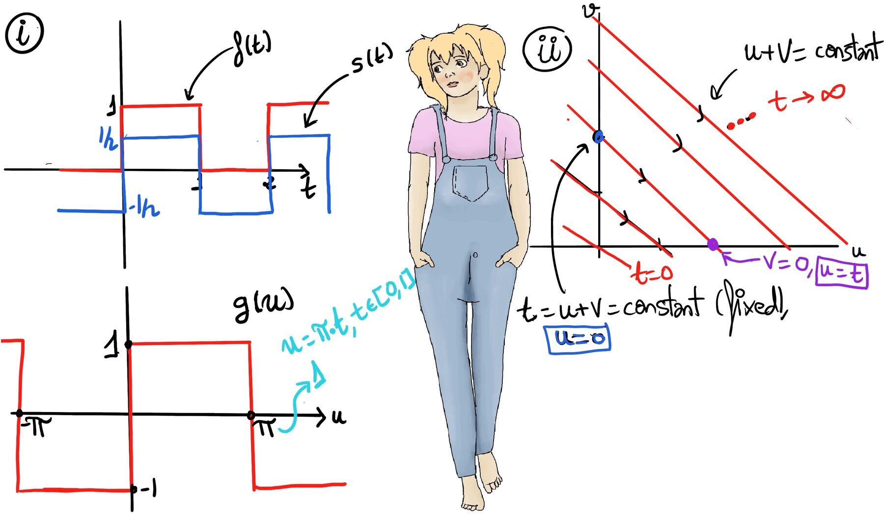
Computing the Fourier series of $f(t)$ directly can be tedious and messy. Instead, we aim to work with an odd function so that all cosine terms vanish, leaving us with a pure sine series.

We can create a new function $s(t)$ by shifting $f(t)$ downward by exactly half its amplitude: $s(t) = f(t) - \frac{1}{2}$

$$s(t) = \begin{cases} 1/2, & 0 < t < 1 \\ -1/2, & 1 < t < 2 \end{cases}$$

This new function $s(t)$ is perfectly symmetric about the origin (an odd function).

To find its Fourier series easily, let’s consider a standard reference function $g(u)$, defined on $(0, \pi)$ and extended to an odd periodic function with period $2\pi$:

$$g(u)= \begin{cases} 1, & 0 < u < \pi \\ -1, & -\pi < u < 0 \end{cases}$$

The Fourier series of this standard odd extension $g(u)$ is a well-known result: $g(u) = \sum_{n=1, \text{ odd}}^\infty \frac{4}{n\pi}\sin(nu) = \frac{4}{\pi}\sum_{n=1, \text{ odd}}^\infty \frac{\sin(nu)}{n}$

Now, to relate our shifted wave $s(t)$ to this reference function $g(u)$, observe that $s(t) = \frac{1}{2}g(u)$ if we set $u = \pi t$. This transformation maps the time interval $t \in [0, 1]$ perfectly to the angular interval $u \in [0, \pi]$.

Substituting $u = \pi t$ back into our equation: $s(t) = \frac{1}{2}g(\pi t) = \frac{1}{2} \left[ \frac{4}{\pi}\sum_{n=1, \text{ odd}}^\infty \frac{\sin(n\pi t)}{n} \right] = \frac{2}{\pi}\sum_{n=1, \text{ odd}}^\infty \frac{\sin(n\pi t)}{n}$

Since our original function was $f(t) = \frac{1}{2} + s(t)$, we can easily write the final Fourier series for our original square wave: $\boxed{f(t) = \frac{1}{2} + \frac{2}{\pi}\sum_{n=1, \text{ odd}}^\infty \frac{\sin(n\pi t)}{n}}$

Step 2. Solving the Differential Equation

We now return and substitute our infinite series back into the original differential equation: $x'' + \omega_0^2x = \frac{1}{2} + \frac{2}{\pi}\sum_{n=1, \text{ odd}}^\infty \frac{\sin(n\pi t)}{n}$

Because the differential operator ($x'' + \omega_0^2x$) is linear, we can use the Principle of Superposition. This means the particular solution to the entire sum of inputs is exactly equal to the sum of the particular solutions for each individual input.

Let’s look at the standard solutions for these individual pieces:

1. The Constant Term (DC Offset): For $x'' + \omega_0^2x = C$, the particular solution is simply $x_p = \frac{C}{\omega_0^2}$.
2. The Sine Terms (AC Harmonics): For $x'' + \omega_0^2x = A\sin(\omega t)$, the particular solution is $x_p = \frac{A\sin(\omega t)}{\omega_0^2 - \omega^2}$.

   We can calculate $x_p$ if the right hand side of the previous equation is either cos(wt), sin(wt), or some multiple of them. The procedure is basically to convert the differential equation in a complex differential equation as we have previously done $x''+ w_o^2x = cos(wt), x''+ w_o^2x = sin(wt)$ and the solution is: $x_p = \frac{cos(wt)}{w_o^2-w^2}, \frac{sin(wt)}{w_o^2-w^2}$ respectively. Notice that if w = 0, the formula still applies: $x_p = \frac{cos(0·t)}{w_o^2-0^2} = \frac{1}{w_o^2}$

By applying these standard solutions to every term in our infinite series (where our input frequency is $\omega_n = n\pi$), we construct the full particular solution.

The Particular Solution $x_p(t)$: $\boxed{x_p(t) = \frac{1}{2\omega_0^2} + \frac{2}{\pi}\sum_{n=1, \text{ odd}}^\infty \frac{\sin(n\pi t)}{n(\omega_0^2 - (n\pi)^2)}}$

Step 3: Analyzing the Solution (The Resonance Phenomenon)

The true power of this mathematical formulation reveals itself when we plug in real numbers. Let’s assume our system has a natural frequency of $\omega_0 = 10$.

Let’s calculate the denominator term, $\omega_0^2 - (n\pi)^2$, for the first few harmonics to see how the system responds to the different frequencies hidden inside the square wave.

Harmonic (n)	Frequency (nπ)	Denominator (100−n2π2)	Resulting Amplitude
$n = 1$	$1\pi \approx 3.14$	$100 - \pi^2 \approx 90.13$	$\frac{2}{\pi} \cdot \frac{1}{1 \cdot 90.13} \approx \mathbf{0.007}$
$n = 3$	$3\pi \approx 9.42$	$100 - 9\pi^2 \approx 11.17$	$\frac{2}{\pi} \cdot \frac{1}{3 \cdot 11.17} \approx \mathbf{0.019}$
$n = 5$	$5\pi \approx 15.70$	$100 - 25\pi^2 \approx -146.74$	$\frac{2}{\pi} \cdot \frac{1}{5 \cdot (-146.74)} \approx \mathbf{-0.00087}$

For n = 5 and higher odd values of n, the denominator becomes negative and large in magnitude.

Expanding the solution with these computed amplitudes yields: $x_p(t) \approx 0.005 + 0.007\sin(\pi t) + 0.019\sin(3\pi t) - 0.00087\sin(5\pi t) + \dots$

The Core Insight

Look closely at the amplitudes. Usually, in a Fourier series, the lowest frequency (the fundamental, $n=1$) is the largest, and the higher harmonics steadily fade away.

However, in this dynamic system, the amplitude of the 3rd harmonic ($0.019$) is nearly three times larger than the fundamental harmonic ($0.007$)!

The terms with n = 1 and n = 3 have significantly larger amplitudes compared to higher n. Thus, the solution shows that the frequencies corresponding to n = 1 (πt) and n = 3 (3πt) are the most significant, as their amplitudes are much larger than the amplitudes of higher frequencies.

When $\omega_0$ is close to one of these frequencies ($\omega_0 \approx \pi$ or $\omega_0 \approx 3\pi$), the denominator $w_o^2-(nπ)^2$ becomes small, causing the amplitude of the corresponding sine term to become large. This is the resonance phenomenon, where the system’s natural frequency $\omega_0$ matches one of the input frequencies, resulting in a large response.

The frequencies in f(t) are hidden, but the system picks out, favors, resonates or responds more strongly (or violently) to the frequencies in the input that are close to its natural frequency (or rhythm). In our example with $\omega_0$ = 10, the frequency $3\pi \approx 9.42$ is close to $\omega_0$, resulting in a larger amplitude for n = 3: 0.019.

Alternative Method: Direct Substitution

Another powerful way to solve $x'' + \omega_0^2x = f(t)$ is to use the method of undetermined coefficients. Because our input force $f(t)$ is expressed as a Fourier sine series with a constant offset, it is reasonable to guess that our particular solution $x_p(t)$ will have the exact same structure.

We assume a particular solution of the form: $x_p(t) = c_0 + \sum_{n=1}^\infty c_n\sin(n\pi t)$ (the solution is similar to the input function) where $c_0$ and $c_n$ are unknown constants we need to find.

Step 1: Differentiate the Assumed Solution

To substitute this guess into our differential equation, we first need to find its second derivative. We differentiate term-by-term with respect to $t$:

1. First derivative: $x_p'(t) = \sum_{n=1}^\infty c_n(n\pi)\cos(n\pi t)$
2. Second derivative: $x_p''(t) = \sum_{n=1}^\infty -c_n(n\pi)^2\sin(n\pi t)$

Step 2: Substitute into the Differential Equation

Recall our original differential equation and the Fourier series representation of our square wave $f(t)$: $x'' + \omega_0^2x = \frac{1}{2} + \frac{2}{\pi}\sum_{n=1, \text{ odd}}^\infty \frac{\sin(n\pi t)}{n}$

Substitute our assumed $x_p(t)$ and $x_p''(t)$ into the left side of the equation: $\left[ \sum_{n=1}^\infty -c_n(n\pi)^2\sin(n\pi t) \right] + \omega_0^2\left[ c_0 + \sum_{n=1}^\infty c_n\sin(n\pi t) \right] = \frac{1}{2} + \frac{2}{\pi}\sum_{n=1, \text{ odd}}^\infty \frac{\sin(n\pi t)}{n}$

Now, distribute $\omega_0^2$ and group the like terms on the left side: $\omega_0^2c_0 + \sum_{n=1}^\infty c_n\left(\omega_0^2 - (n\pi)^2\right)\sin(n\pi t) = \frac{1}{2} + \sum_{n=1, \text{ odd}}^\infty \frac{2}{n\pi}\sin(n\pi t)$

Step 3: Match Coefficients

For this equation to hold true for all values of $t$, the coefficients of corresponding terms on both sides of the equals sign must be identical. We can match them up:

1. The Constant Terms:
   $$\omega_0^2c_0 = \frac{1}{2} \quad \implies \quad c_0 = \frac{1}{2\omega_0^2}$$
2. The Sine Terms (for even $n$):
   The right side of the equation has no even $n$ terms (they are zero). Therefore, $c_n\left(\omega_0^2 - (n\pi)^2\right) = 0 \quad \implies \quad c_n = 0 \text{ (for all even } n)$
   I need to flag one particular caveat. We are assuming that $\omega_0^2 \ne (n\pi)^2$. Otherwise, we’re in a resonant situation and we need a modified particular solution.
3. The Sine Terms (for odd $n$):
   Match the coefficients for the odd harmonics: $c_n\left(\omega_0^2 - (n\pi)^2\right) = \frac{2}{n\pi}$.
   Solving for $c_n$ gives us: $c_n = \frac{2}{n\pi\left(\omega_0^2 - (n\pi)^2\right)}$

Step 4: Final Result

Substitute the derived coefficients ($c_0$ and $c_n$) back into our original assumed solution $x_p(t)$. Since $c_n = 0$ for all even values of $n$, we only sum over the odd indices: $x_p(t) = \frac{1}{2\omega_0^2} + \sum_{n=1, \text{ odd}}^\infty \frac{2\sin(n\pi t)}{n\pi\left(\omega_0^2 - (n\pi)^2\right)}$

Factoring out the constants yields, $x_p(t) = \frac{1}{2\omega_0^2} + \frac{2}{\pi}\sum_{n=1, \text{ odd}}^\infty \frac{\sin(n\pi t)}{n(\omega_0^2 - (n\pi)^2)}$

This confirms that the Direct Substitution method perfectly matches the result we found earlier using the Superposition Principle.

Bibliography

1. NPTEL-NOC IITM, Introduction to Galois Theory.
2. Algebra, Second Edition, by Michael Artin.
3. LibreTexts, Calculus and Calculus 3e (Apex). Abstract and Geometric Algebra, Abstract Algebra: Theory and Applications (Judson).
4. Field and Galois Theory, by Patrick Morandi. Springer.
5. Michael Penn, and MathMajor.
6. Contemporary Abstract Algebra, Joseph, A. Gallian.
7. YouTube’s Andrew Misseldine: Calculus. College Algebra and Abstract Algebra.
8. MIT OpenCourseWare [18.03 Differential Equations, Spring 2006], YouTube by MIT OpenCourseWare.
9. Calculus Early Transcendentals: Differential & Multi-Variable Calculus for Social Sciences.