Linear and Autonomous First-Order Systems of ODEs

All things are difficult before they are easy, Thomas Fuller.

When you have eliminated the impossible, whatever remains, however improbable, must be the truth, Sherlock Holmes.

General Form of a First-Order System

Many complex physical systems cannot be described by a single variable changing over time. Instead, they involve multiple interacting components. We model these interactions using a system of Ordinary Differential Equations (ODEs).

A general first-order system with two dependent variables, $x(t)$ and $y(t)$, takes (or can be written in) the general form:

$\begin{cases} x' = f(x, y, t) \\ y' = g(x, y, t) \end{cases}$ where

• $x'$ and $y'$ represent the time derivatives $\frac{dx}{dt}$ and $\frac{dy}{dt}$ respectively.
• $f$ and $g$ are functions describing how $x$ and $y$ change based on the current state of both variables, and possibly the independent variable t.

Linear First-Order Systems

In a linear system, the dependent variables $x(t)$ and $y(t)$ only appear to the first power, meaning that the equations do not contain any nonlinear terms such as $x^2$, $x \cdot y$, or $\sin(x)$. The coefficients of x and y can be functions of t, but the variables themselves are not multiplied together or raised to any power other than one.

The general form of a linear first-order system is:

$\begin{cases} x' = a(t)x + b(t)y + r_1(t) \\ y' = c(t)x + d(t)y + r_2(t) \end{cases}$ where:

• $a(t), b(t), c(t), d(t)$ are time-dependent coefficients (often just constants).
• $r_1(t)$ and $r_2(t)$ are external forcing functions or inputs.
• $x(t_0) = x_0$ and $y(t_0) = y_0$ are the initial conditions, indicating the values of x and y at some initial time $t_0$.

Characteristics of Linear Systems

• Linearity: The dependent variables x(t) and y(t) occur linearly in the equations.
• Homogeneous vs. Nonhomogeneous: If both $r_1(t) = 0$ and $r_2(t) = 0$, there are no external forces, the system is called a homogeneous linear system. The system’s evolution is entirely determined by its internal state.
  If either $r_1(t)$ or $r_2(t)$ is non-zero, the system is being actively driven by an outside force, the system is nonhomogeneous.
  💡 Note: Homogeneous systems are mathematically foundational because their natural solutions are used to construct the solutions for nonhomogeneous systems.

Example: Modeling Temperature Dynamics in an Egg

To illustrate how we can apply a first-order system of ODEs, consider the following physical scenario:

Consider an egg consisting of two interacting regions:

• The Yolk: The inner part or core with temperature $T_1(t)$.
• The Egg White: The surrounding layer with temperature $T_2(t)$.

Supposed the egg is placed in a pot of water. Initially, the water is boiling (the egg is cooked), but it cools over time, especially when the egg is transferred to an ice bath (the external environment) with temperature $T_e$. Refer to Figure iv for a visual representation and aid in understanding it.

We aim to model the temperature dynamics of the yolk and egg white over time using a first-order system of ODEs.

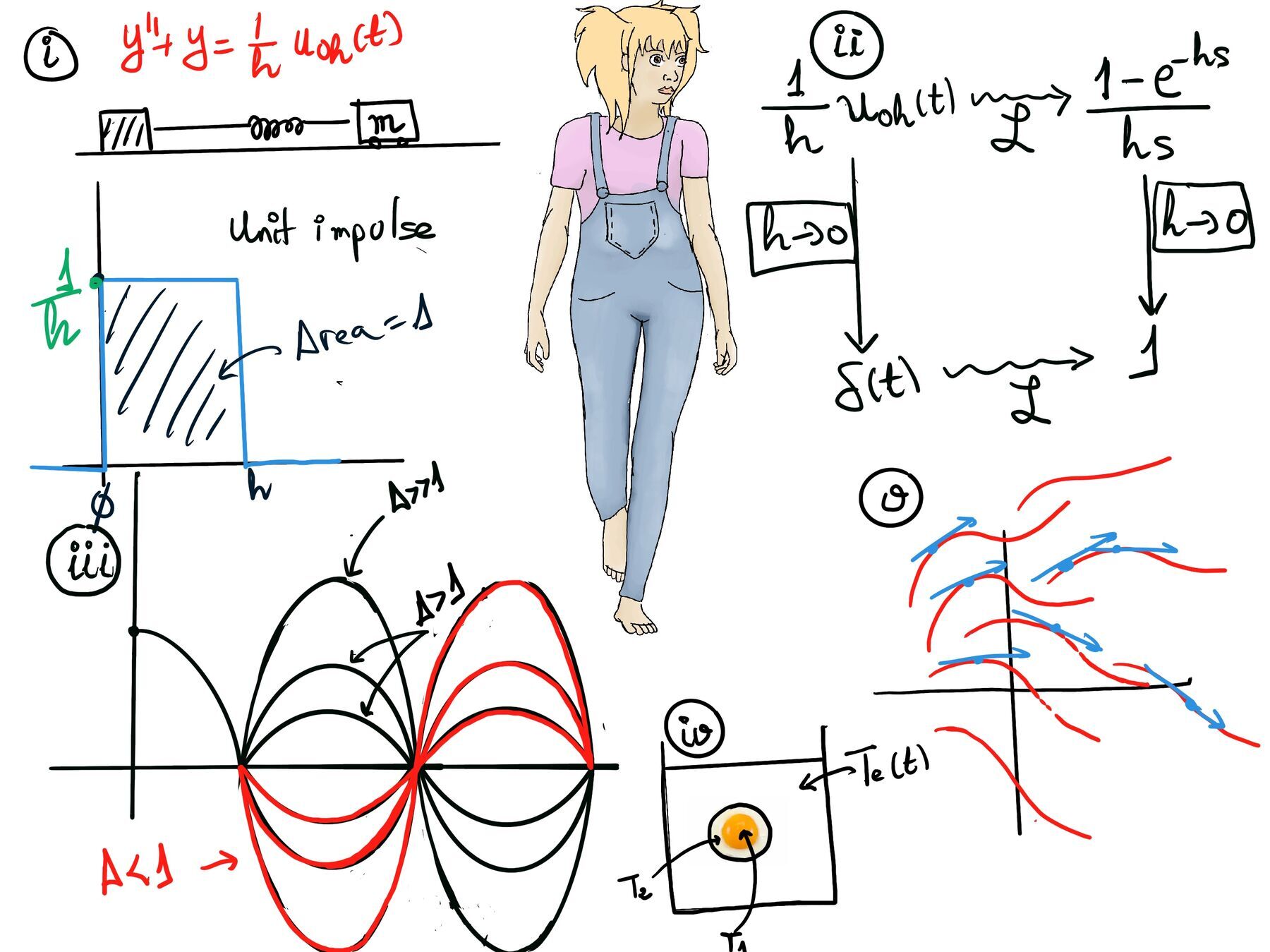
The temperature of the water is modeled as: $T_e(t) = 100\cdot e^{-kt}$ for some positive constant k, meaning the water cools over time and decays exponentially. For simplicity, we assume $T_e(t) = 0^\circ \text{C}$ when the egg is transferred to an ice bath.

The initial temperatures of the egg are $T_1(0) = 40^\circ \text{C}$ (yolk) and $T_2(0) = 45^\circ \text{C}$ (white).

To model the temperature dynamics of the egg, we use Newton’s Law of Cooling, which states that the rate of change of temperature is proportional to the temperature difference between between the object and its immediate surroundings.

Formulating the System

Using Newton’s Law of Cooling, we can model the temperature changes as:

1. Yolk Temperature Change: The yolk only touches the egg white. The rate of temperature change of the yolk depends on the temperature difference between the egg white and the yolk: $\frac{dT_1}{dt} = a(T_2-T_1)$
2. Egg White Temperature Change. The rate of temperature change of the egg white depends on:

• The temperature difference between the yolk and the egg white.
• The temperature difference between the external environment and the egg white.

$\frac{dT_2}{dt} = a(T_1-T_2) + b(T_e-T_2)$ where:

• $T_1(t)$ is the temperature of the yolk
• $T_2(t)$ is the temperature of the egg white.
• a and b are positive constants that describe the rates of heat transfer between the yolk and egg white, and between the egg white and the external environment (water).
• $T_e(t)$ is the external temperature (the pot of water or ice bath).

For this particular example, let’s assume a = 2 (heat transfer between the yolk and white), b = 3 (heat transfer between the egg white and the external environment). Initial conditions: $T_1(0) = 40^\circ \text{C}$ (yolk) and $T_2(0) = 45^\circ \text{C}$ (egg white). Since the ice bath is at $0^\circ \text{C}$, $T_e = 0$.

Plugging these values in, we get our specific linear system:

$\begin{cases} T_1' = -2T_1 + 2T_2 \quad \text{(i)} \\ T_2' = 2T_1 - 5T_2 \quad \text{(ii)} \end{cases}$

Solving the System

We can solve this system using the method of substitution (converting the first-order system into a single second-order ODE).

1. Isolate $T_2$ from equation (i).
   From $T_1' = -2T_1 + 2T_2$, we can solve for $T_2$: $2T_2 = T_1' + 2T_1 \implies T_2 = 0.5T_1' + T_1$

2. Differentiate to find $T_2'$. $T_2' = 0.5T_1'' + T_1'$

3. Substitute $T_2$ and $T_2'$ into equation (ii).
   Take equation (ii): $T_2' = 2T_1 - 5T_2$ and plug in our $T_1$ equivalents: $0.5T_1'' + T_1' = 2T_1 - 5(0.5T_1' + T_1)$.
   $0.5T_1'' + T_1' = 2T_1 - 2.5T_1' - 5T_1$
   Group all terms on one side: $0.5T_1'' + 3.5T_1' + 3T_1 = 0$
   Multiply by $2$ to clear decimals: $T_1'' + 7T_1' + 6T_1 = 0$

4. Solve the Second-Order ODE. This is now a second-order linear differential equation. In general, a system of two first-order differential equations, will produce a second-order differential equation by substitution. A system of three first-order differential equations, will produce a third-order differential equation, and so on.
   The equation $T_1'' + 7T_1' + 6T_1 = 0$ is a standard linear homogeneous ODE. The characteristic equation associated with the ODE is: $r^2 + 7r + 6 = 0$. Factor this equation: $r^2 + 7r + 6 = (r + 1)(r + 6)$. The roots or solutions of this characteristic equation are -1 and -6.
   Therefore, the solution for the yolk temperature is: $T_1 = C_1e^{-t} + C_2e^{-6t}$ where $C_1$ and $C_2$ are constants to be determined from initial conditions.

5. Find $T_2(t)$. Recall from Step 1 that $T_2 = 0.5T_1' + T_1$. Calculate $T_1'(t)$, $T_1'(t) = -C_1e^{-t} - 6C_2e^{-6t}$.
   Now substitute into the $T_2$ formula: $T_2(t) = 0.5(-C_1e^{-t} - 6C_2e^{-6t}) + (C_1e^{-t} + C_2e^{-6t})$
   Simplify, $T_2(t) = 0.5C_1e^{-t} - 2C_2e^{-6t}$

6. Apply Initial Conditions. We know $T_1(0) = 40$ and $T_2(0) = 45$.
   So $C_1 + C_2 = 40$ (i) and $0.5C_1 - 2C_2 = 45$ (ii).
   Multiply the second equation by 2: $C_1 - 4C_2 = 90$.
   Subtract this from the first equation: $(C_1 + C_2) - (C_1 - 4C_2) = 40 - 90$
   $5C_2 = -50 \implies C_2 = -10$.
   Since $C_1 + C_2 = 40$ (i), we know $C_1 - 10 = 40 \implies C_1 = 50$.

7. The Final Solution.
   The temperature dynamics of the egg over time are given exactly by:
   $T_1(t) = 50e^{-t} - 10e^{-6t} \quad \text{(Yolk)}$
   $T_2(t) = 25e^{-t} + 20e^{-6t} \quad \text{(Egg White)}$

8. Intuition. The equations perfectly capture the physics of the scenario.
   The egg white ($T_2$) is in direct contact with the $0^\circ\text{C}$ ice bath. It cools rapidly by losing heat directly to the environment.
   The yolk ($T_1$), however, is insulated. It can only lose heat to the egg white. Because the egg white acts as a buffer, the yolk's temperature decreases more gradually.
   Eventually, as $t \to \infty$, both the fast-decaying term ($e^{-6t}$) and the slow-decaying term ($e^{-t}$) vanish, and the entire egg reaches thermal equilibrium with the $0^\circ\text{C}$ ice bath.

Solving a System of First-Order Linear ODEs (Operator Method)

Consider the following coupled system:

$\begin{cases} x' + y' + 2x = 0 \\ x' + y' - x - y = \sin(t) \end{cases}$

To solve this systematically, we use the Differential Operator Method. We define the operator $D = \frac{d}{dt}$. Applying this operator turns our calculus problem into an algebra problem.

1. Standardize with the $D$ Operator.
   Rewrite the system by grouping the $x$ and $y$ variables and factoring out the operations:
   

   $$\begin{cases} (D + 2)x + Dy = 0 \quad \text{(Eq. 1)} \\ (D - 1)x + (D - 1)y = \sin(t) \quad \text{(Eq. 2)} \end{cases}$$

2. Eliminate a Variable ($y$).
   To solve the system, we aim to eliminate one of the variables, allowing us to find an expression for the other. Here’s how we can proceed.
   Multiply Equation 1 by $(D - 1)$: $(D - 1)(D + 2)x + (D - 1)Dy = 0$
   Multiply Equation 2 by $-D$: $-D(D - 1)x - D(D - 1)y = -D(\sin(t))$
   The reader should notice that $-D(\sin(t))$ simply means taking the negative derivative of $\sin(t)$, which is $-\cos(t)$.
   Now, add the two equations together. The $y$ terms perfectly cancel out! $(D^2 + D - 2)x - (D^2 - D)x = -\cos(t)$
   Simplify the operators on $x$: $(D^2 - D^2 + D - (-D) - 2)x = -\cos(t)$
   $(2D - 2)x = -\cos(t)$
   Finally, translate this back from operator notation to standard notation $2x' - 2x = -\cos(t) \implies[\text{Divide by 2}] x' - x = -0.5\cos(t)$

3. Solve for $x(t)$ Using an Integrating Factor.
   $x' - x = -0.5\cos(t)$ is a standard first-order linear ODE: $x' + P(t)x = Q(t)$.
   Find the Integrating Factor: $\mu(t) = e^{\int -1 dt} = e^{-t}$
   Multiply both sides by $\mu(t)$: $e^{-t}x' - e^{-t}x = -0.5e^{-t}\cos(t)$
   $\frac{d}{dt}(e^{-t}x) = -0.5e^{-t}\cos(t)$
   Integrate both sides: $e^{-t}x = -0.5 \int e^{-t}\cos(t) dt + C_1$
   Using the standard integral formula $\boxed{\int e^{at}\cos(bt) dt = \frac{e^{at}(a\cos(bt) + b\sin(bt))}{a^2 + b^2}}$, where $a = -1$ and $b = 1$: $e^{-t}x = -0.5 \left( \frac{e^{-t}(-\cos(t) + \sin(t))}{2} \right) + C_1$.
   $e^{-t}x = \frac{1}{4}e^{-t}(\cos(t) - \sin(t)) + C_1$
   Next, we multiply through by $e^t$ to isolate $x(t)$: $x(t) = C_1e^t + \frac{1}{4}\cos(t) - \frac{1}{4}\sin(t)$

4. Solve for $y(t)$.
   First, we calculate $x'(t)$: $x'(t) = C_1e^t - \frac{1}{4}\sin(t) - \frac{1}{4}\cos(t)$
   Use the simplest original equation (Equation 1: $x' + y' + 2x = 0$) to find $y'$: $y' = -x' - 2x$
   $y' = -\left(C_1e^t - \frac{1}{4}\sin(t) - \frac{1}{4}\cos(t)\right) - 2\left(C_1e^t + \frac{1}{4}\cos(t) - \frac{1}{4}\sin(t)\right)$
   $y' = -3C_1e^t + \frac{3}{4}\sin(t) - \frac{1}{4}\cos(t)$
   Integrate to find $y(t)$: $y(t) = -3C_1e^t - \frac{3}{4}\cos(t) - \frac{1}{4}\sin(t) + C_2$

5. Verify and Eliminate Extraneous Constant.
   💡 The Trap: The elimination method frequently introduces “extraneous” constants when we integrate. Our combined ODE for $x$ was first-order ($2x' - 2x = -cos(t)$), meaning the entire system only possesses one true degree of freedom. Therefore, $C_2$ cannot be arbitrary!
   To find the restriction on $C_2$, we must plug our $x(t)$ and $y(t)$ back into Equation 2: $x' + y' - x - y = \sin(t)$.
   We know (equation 1) $x' + y' = -2x = -2C_1e^t - 0.5\cos(t) + 0.5\sin(t)$
   We calculate $-x - y = -(C_1e^t + \frac{1}{4}\cos(t) - \frac{1}{4}\sin(t)) -(-3C_1e^t - \frac{3}{4}\cos(t) - \frac{1}{4}\sin(t) + C_2) = 2C_1e^t + 0.5\cos(t) + 0.5\sin(t) - C_2$
   Add them together (equation 2): $(-2C_1e^t - 0.5\cos(t) + 0.5\sin(t)) + (2C_1e^t + 0.5\cos(t) + 0.5\sin(t) - C_2) = \sin(t)$
   Simplify, $\sin(t) - C_2 = \sin(t)$. Therefore, $C_2 = 0$.

6. The Final True Solution.

$$\begin{cases} x(t) = C_1e^t + \frac{1}{4}(\cos(t) - \sin(t)) \\ y(t) = -3C_1e^t - \frac{1}{4}(3\cos(t) + \sin(t)) \end{cases}$$

Autonomous Systems of First-Order ODEs

An autonomous system is a system of differential equations where the independent variable, typically denoted by t (often representing time), does not explicitly appear on the right-hand side of the equations. In other words, the rate of change of the dependent variables depends only on the current state of the system, not directly on time.

General Form

A system of two first-order autonomous ODEs can be written as:

$\begin{cases} x' = f(x, y) \\ y' = g(x, y) \end{cases}$ where:

• $x(t)$ and $y(t)$ are the dependent variables, functions of the independent variable t.
• x’ = $\frac{dx}{dt}$ and y’ = $\frac{dy}{dt}$ represent the time derivatives of the function x(t) and y(t), respectively.
• The functions f(x, y) and g(x, y) determine how x(t) and y(t) evolve over time (change) based exclusively on their current state $(x, y)$.

Key Characteristics of Autonomous Systems

1. Time-Invariant Behavior: Since t does not explicitly appear in f and g, the rules of the system never change. In other words, the system’s behavior (and how it evolves) is the same at any time t, given the same state (x, y).
2. Dependence on State: The evolution of the system depends solely on the current state (x, y), making the system’s behavior consistent across time. Hence, we can graph the entire behavior of the system on an $xy$-coordinate plane (called the Phase Plane), entirely ignoring the $t$ axis!

Equilibrium Points (Critical Points)

The most important feature of an autonomous system is its equilibrium points. An equilibrium point $(x_0, y_0)$ occurs where the system is completely at rest —meaning the rates of change are zero: $f(x_0, y_0) = 0 \quad \text{and} \quad g(x_0, y_0) = 0$

If a system reaches an equilibrium point, it will stay there forever (since $x' = 0$ and $y' = 0$). Analyzing whether these points are stable (attracting nearby states) or unstable (repelling nearby states) is the core of modern dynamical systems theory, allowing us to predict long-term behavior without ever actually solving the differential equations!

Solutions as Parametrized Curves in the Plane

When we solve an autonomous system, we find two functions $x(t)$ and $y(t)$. Instead of graphing these separately against time, we can plot them together as a parametrized curve in the $xy$-plane $\mathbb{R}^2$, meaning that for each value of t, there is a corresponding point (x(t), y(t)) in the plane. As t varies, the point (x(t), y(t)) traces out a curve.

Each solution to the system corresponds to a different initial condition $x(t_0) = x_0, y(t_0) = y_0$ where $t_0$ is the initial time (often $t_0 = 0$) and ($x_0, y_0$) is the initial point in the plane (Refer to Figure v for a visual representation and aid in understanding it).

For every moment in time $t$, there is a corresponding point $(x(t), y(t))$. As time varies, this point traces out a continuous path called a trajectory, orbit, or solution curve.

Implications

1. Initial Conditions dictate the Starting Point: A specific solution corresponds to an Initial Value Problem (IVP) where $x(t_0) = x_0$ and $y(t_0) = y_0$. This $(x_0, y_0)$ coordinate is simply the starting location in the plane where the curve begins drawing.
2. Unique, Non-Intersecting Paths: Provided the functions $f(x, y)$ and $g(x, y)$ are smooth and continuous, trajectories can never intersect each other. If two curves crossed, the system would have two different valid directions to travel from a single point, which violates the mathematical uniqueness of differential equations.
3. Family of Solutions: By varying the initial condition $(x_0, y_0)$, we generate an infinite family of solution curves, each representing a different trajectory in the plane. Plotted together, these map out the complete geometric behavior of the system across the entire plane.

The Velocity Field Interpretation

We can understand and visualize an autonomous system without ever calculating the analytical solution by treating the ODEs as a Velocity Field.

The system of ODEs: $\begin{cases} x' = f(x, y) \\\ y' = g(x, y) \end{cases}$ defines a velocity field in the plane. At each point (x, y), the system assigns a precise 2D vector $\vec{v}(x, y) = \langle f(x, y), g(x, y) \rangle$ to every single point $(x, y)$ in the plane.

🌊 The Fluid Flow Analogy.

Imagine the Phase Plane is the surface of a river. The vector field tells you the exact speed and direction the water is flowing at any given coordinate. Finding the solution to the differential equation is mathematically equivalent to dropping a leaf (the initial condition) onto the water at $(x_0, y_0)$ and predicting the path (the trajectory) it gets swept along!

Anatomy of the Velocity Field:

• Direction and Magnitude: The vector $\vec{v}(x,y)=(f(x,y),g(x,y))$ indicates the direction and speed (magnitude) at which the system moves when it is at the point (x, y). It dictates exactly which way the system is heading and how fast. The speed (magnitude) at any point is $\sqrt{(x')^2 + (y')^2}$.
• Tangent Vectors: Because $x'$ and $y'$ are literally the time-derivatives of position, the assigned vector at any point $(x, y)$ is always perfectly tangent to the solution curve passing through that coordinate.
• The plane $\mathbb{R}^2$ where x and y are plotted is called the phase plane.

Therefore, a system of two first order autonomous ODE is fundamentally identical to a velocity field. The true analytical solutions are simply the continuous parametric curves that flawlessly follow the arrows of the field, moving strictly in the direction and speed specified by the flow at every single point.

Bibliography

1. NPTEL-NOC IITM, Introduction to Galois Theory.
2. Algebra, Second Edition, by Michael Artin.
3. LibreTexts, Calculus and Calculus 3e (Apex). Abstract and Geometric Algebra, Abstract Algebra: Theory and Applications (Judson).
4. Field and Galois Theory, by Patrick Morandi. Springer.
5. Michael Penn, and MathMajor.
6. Contemporary Abstract Algebra, Joseph, A. Gallian.
7. YouTube’s Andrew Misseldine: Calculus. College Algebra and Abstract Algebra.
8. MIT OpenCourseWare [18.03 Differential Equations, Spring 2006], YouTube by MIT OpenCourseWare.
9. Calculus Early Transcendentals: Differential & Multi-Variable Calculus for Social Sciences.