
|
 |

|
|
|
|
|
|
Being happy doesn’t mean that everything is perfect. It means you’ve decided to look beyond the imperfections, Anonymous.
An algebraic equation is a mathematical statement asserting that two algebraic expressions are equal.. These expressions are constructed using:
An algebraic equation typically has the following general form: Expression1 = Expression2, where the two expressions are set equal to each other.
Examples: y = 2x + 4 (simple linear equation, represents a straight line with a slope of 2 and a y-intercept of 4), ax2 + bx + c = 0 (quadratic equation, it represents a parabola), $ln(xy + t) = z·sin(\sqrt{x})$.
Definition. A differential equation is an equation that involves one or more functions and their derivatives. It relates the function itself (the dependent variable), its derivatives with respect to one or more independent variables (rates of change), and the independent variable(s) themselves, e.g., $\frac{dy}{dx} = 3x +5y, y' + y = 4xcos(2x), \frac{dy}{dx} = x^2y+y, etc.$
If an algebraic equation is a “snapshot” of a relationship, a differential equation is the “instruction manual” for how that relationship moves and changes.
Key Components (e.g., $\frac{dy}{dx} = 3x +5y$):
First-order linear differential equations are fundamental tools in mathematical modeling across various disciplines, including physics, engineering, biology, and economics. They are used to describe dynamic systems where the rate of change of a quantity depends linearly on the quantity itself and, frequently, on external inputs.
Definition. A first-order linear ordinary differential equation is an ordinary differential equation (ODE) involving an unknown function y(x), its first derivative y′, and functions of the independent variable x, which can be written in the general form:: a(x)y' + b(x)y = c(x) where:
These equations are termed “linear” because the unknown function y and its derivative y’ strictly appear to the first power. They are never multiplied together, squared, or composed inside nonlinear functions (like sin(y) or $e^y$).
If the forcing function c(x) = 0 for all x in the interval of interest, the equation simplifies to: a(x)y’ + b(x)y = 0. Such an equation is called a homogeneous linear differential equation. If $c(x) \ne 0$, it is non-homogeneous.
To standardize the equation and prepare it for universal solution methods, we divide both sides of the general form by a(x), assuming a(x) ≠ 0: y’ + p(x)y = q(x) where $p(x)=\frac{b(x)}{a(x)}\text{ and }q(x) = \frac{c(x)}{a(x)}$ This is the standard linear form of a first-order differential equation, which is more convenient for applying solution methods, such as the integrating factor method.

First-order linear differential equations with periodic inputs are incredibly common in modeling physical systems subjected to continuous oscillatory forces. Examples include electrical circuits driven by alternating currents (AC), structural systems experiencing cyclic mechanical vibrations, or environmental models with seasonal temperature fluctuations.
Consider the standard first-order linear differential equation: $\frac{dy}{dt} + ky = kq_e(t)$ where:
Our goal is to find the explicit solution y(t) that dictates how the system responds to this oscillating drive.
Solving this equation using standard real-number integration techniques (like integration by parts) is notoriously tedious and error-prone because of the integral $e^{kt}cos(wt)$.
Instead, we use a brilliant mathematical shortcut: complexification. The core idea is that complex exponentials (of the form $e^{i\theta}$) are easier to work with than trigonometric functions. Once we solve the complex version of the equation, we can extract the real part to find the solution to the original problem, $cos(wt) = \mathbb{Re}(e^{iwt})$.
By utilizing Euler’s formula, $e^{iwt} = cos(wt) + isin(wt)$, we can upgrade our real differential equation into a complex one: $\tilde{y'}+k\tilde{y} = ke^{iwt}$, where $\tilde{y}(t)= y_1(t) + iy_2(t)$ is a complex-valued function. Because the differential operator is linear, our strategy is incredibly elegant: solve the complex differential equation for $\tilde{y}$, and then simply extract the real part of the answer to obtain the solution to our original, real-world, differential equation ODE. Since the real part of the complex input $e^{iwt}$ is kcos(wt), the real part of the complex output $\tilde{y}$ will be our desired y(t).
The complex differential equation is a standard first-order linear differential equation and can be solved swiftly using the integrating factor method: $\tilde{y'}+k\tilde{y} = ke^{iwt}$.
Calculus Reminder. The integral of eat with respect to t is $\frac{1}{a}e^{at}$. Here, our constant a is the complex number k + iw.
Since we are primarily interested in the steady-state solution (long-term behavior), we analyze the transient term $Ce^{-kt}$. Because k > 0, the term decays exponentially and vanishes completely as $t \to \infty$. Thus, we can drop it by setting C=0. The steady-state complex solution is:: $\tilde{y}_{ss} = \frac{1}{1+i(\frac{w}{k})}e^{iwt}$
We want to express the coefficient $\frac{1}{1+i(\frac{w}{k})}$ in a more useful form. We are going to convert this expression to polar form to better understand the magnitude and phase of the solution and extract its real part.
To separate the real and imaginary parts of our solution, we must convert the complex coefficient into polar form.
Recall that any complex number α = x + iy can be expressed in polar form $\alpha = re^{i\phi}$ where:
Besides, $\frac{1}{α}·α = 1 ⇒ |\frac{1}{α}|·|α| = |1| = 1 ⇒ |\frac{1}{α}| = \frac{1}{|α|}, arg(\frac{1}{α})+arg(α) = arg(1) = 0 ⇒ arg(\frac{1}{α}) = -arg(α)$
We are searching for the polar form of $\alpha = 1 + i(\frac{w}{k})$. It has x = 1 (real part), y = w/k (imaginary part)
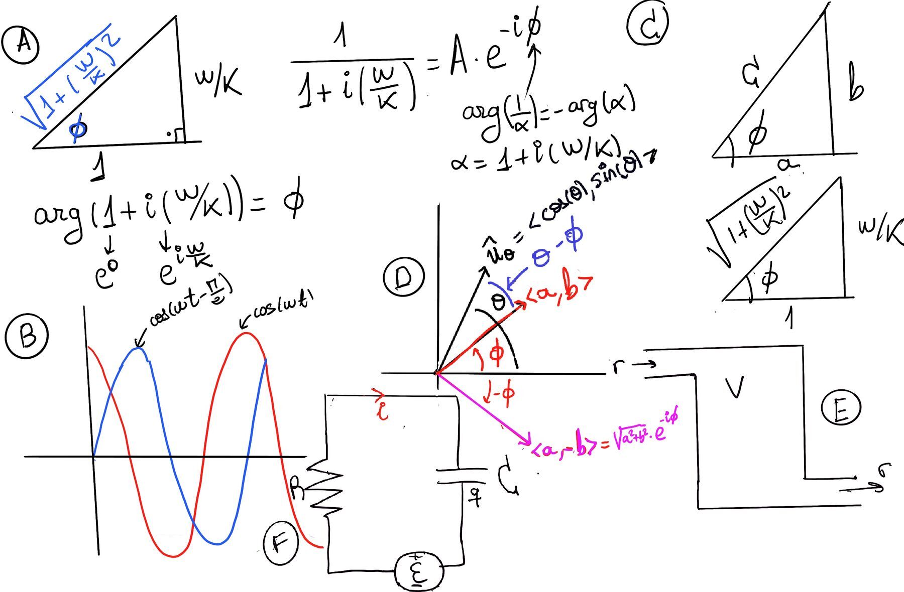
Magnitute: $|\alpha| = \sqrt{1^2 + (\frac{w}{k})^2}$ and phase $\phi = arg(α) = tan^{-1}(\frac{w \ k}{1}) = tan^{-1}(\frac{w}{k})$ (Refer to Figure A for a visual representation and aid in understanding it); we can rewrite it in polar form $ \frac{1}{1+i(\frac{w}{k})} = Ae^{-i\phi} = \frac{1}{\sqrt{1+(\frac{w}{k})^2}}e^{-i\phi}$
Substitute this back into our steady-state equation: $\tilde{y}_{ss}(t) = \frac{1}{1+i(\frac{w}{k})}e^{iwt} = \frac{1}{\sqrt{1+(\frac{w}{k})^2}}e^{iwt-iΦ} = \frac{1}{\sqrt{1+(\frac{w}{k})^2}}e^{i(wt-Φ)}$
Finally, apply Euler’s formula to expand $e^{i(wt-Φ)}$ and take strictly the real part to find our physical steady-state solution: $\boxed{y(t) = \frac{1}{\sqrt{1+(\frac{w}{k})^2}}cos(wt-Φ)}$ where $\phi = tan^{-1}(\frac{w}{k})$ is the phase lag of the function (Refer to Figure B for a visual representation and aid in understanding it).
Our final mathematical solution yields three massive physical insights into how oscillating systems behave:
1. The Forcing Term.
A forcing term in a differential equation represents an external influence or input to the system. In the equation y′ + ky = kcos(ωt), the right side, kcos(ωt), is the forcing term. It represents an external periodic disturbance (e.g., a mechanical vibration, an alternating electric current, or any other cyclical influence on the system) with frequency ω driving the system. It represents an external oscillation with frequency w that forces the system to oscillate as well. If there were no forcing term (y′ + ky = 0), the system would naturally settle into some kind of equilibrium or decay to zero over time.
2. Amplitude Attenuation. The amplitude of the solution is $\frac{1}{\sqrt{1+(\frac{w}{k})^2}}$. Notice that this value is always less than 1.
Damping & Speed: In $\frac{dy}{dt} + ky = k·cos(wt)$, k represents the speed or damping strength of the system. A higher k means the system strongly resists straying from the input and “snaps” to it quickly.
($\star$) If k is very large ($k \to \infty$), the denominator approaches $\sqrt{1 + 0} = 1$, the system’s amplitude matches the input amplitude almost perfectly (the output tracks the input almost perfectly).
($\star$) If ω is very fast (faster oscillations), or k is very weak, the denominator grows massive, causing the system’s physical amplitude to shrink toward zero and the solution responds more slowly to the input. The system’s response lags behind the input by up to 90°. Higher frequency inputs cause the system to lose energy and fail to keep up, resulting in a severely muted physical response.
3. The Phase Lag ($\phi$).
The phase lag $\phi = tan^{-1}(\frac{w}{k})$ indicates how much the system's physical response lags behind the external driving force cos(wt).
In Phase: As $k \to \infty$ (a very fast/stiff system) or $w \to 0$ (a very slow input), $\frac{w}{k} \to 0 \implies \phi = 0$. The system perfectly tracks the input with zero delay.
Out of Phase: As the input frequency speeds up ($w \to \infty$), the ratio $\frac{w}{k} \to \infty$, pushing the phase lag $\phi = \frac{\pi}{2}$ radians (90°). The system’s response falls completely behind the driving force.
While the polar form provides an immediate, intuitive grasp of the amplitude and phase shift, we can reach the exact same conclusion using a purely algebraic method. This alternative approach involves explicitly breaking the complex coefficient down into its Cartesian form (separating the real and imaginary parts) and leveraging a classic trigonometric identity.
Recall our complex steady-state solution to y’ + ky = kcos(wt): $\tilde{y} = \frac{1}{1+i(\frac{w}{k})}e^{iwt}$. The goal is to convert this complex solution into Cartesian form and extract the real part, which gives the solution to the original differential equation.
The expression $\frac{1}{1+i(\frac{w}{k})}$ is a complex fraction. We want to simplify it into a form that separates the real and imaginary parts.
To do this, we rationalize the denominator by multiplying both the numerator and the denominator by the complex conjugate of the denominator, $\frac{1}{1+i(\frac{w}{k})}·\frac{1-i(\frac{w}{k})}{1-i(\frac{w}{k})} = \frac{1-i(\frac{w}{k})}{1+(\frac{w}{k})^2}$
Now, substitute this back into our solution and expand $e^{iwt}$ using Euler’s formula: $\tilde{y} = \frac{1}{1+i(\frac{w}{k})}e^{iwt} = \frac{1-i(\frac{w}{k})}{1+(\frac{w}{k})^2}(cos(wt)+isin(wt))$
Since the original differential equation represents a real physical system, we are only interested in the real part of $\tilde{y}=y_1+iy_2$. We extract the real components by multiplying the real parts together and the imaginary parts together (since i⋅i = −1): $y_1 = \frac{1}{1+(\frac{w}{k})^2}(cos(wt)+\frac{w}{k}sin(wt))$
Using the trigonometry identity $a\cos(\theta) + b\sin(\theta) = c\cos(\theta -\phi)$ where a and b are the two legs or sides of a right triangle, c is the hypotenuse, $\phi$ is the angle between leg a and the hypotenuse c, $\phi = tan^{-1}(\frac{b}{a})$ (Refer to Figure C for a visual representation and aid in understanding it)
$y_1 = \frac{1}{1+(\frac{w}{k})^2}(cos(wt)+\frac{w}{k}sin(wt)) = \frac{1}{1+(\frac{w}{k})^2}·\sqrt{1+(\frac{w}{k})^2}cos(wt-\phi) = (1+(\frac{w}{k})^2)^{-1+\frac{1}{2}}cos(wt-\phi) = \boxed{\frac{1}{\sqrt{1+(\frac{w}{k})^2}}cos(wt-\phi)}$ where $\phi = tan^{-1}(\frac{b}{a}) = tan^{-1}(\frac{w / k}{1}) =tan^{-1}(\frac{w}{k})$ is the phase shit or phase lag, and $\frac{1}{\sqrt{1+(\frac{w}{k})^2}}$ is the amplitude of the oscillation.
This matches the solution obtained using the polar form exactly, confirming that both mathematical paths are valid!
To rigorously justify the formula $a\cos(\theta) + b\sin(\theta) = c\cos(\theta -\phi)$ where a and b are the two legs or sides of a right triangle, c is the hypotenuse, $\phi$ is the angle between a and c, $\phi = tan^{-1}(\frac{b}{a})$, we can prove it using two incredibly elegant methods: Vector Geometry and Complex Arithmetic.
Proof 1: The Vector Dot Product (Geometric Interpretation)
Consider two vectors on a 2D Cartesian plane:
A rotating unit vector $\hat{\mathbf{u}} = ⟨cos(θ), sin(θ)⟩$. Its magnitude is 1, and its angle from the x-axis is $\theta$.
A static coefficient vector $\vec{v}$ = ⟨a, b⟩ with components a and b. Its magnitude is $c = \sqrt{a^2 + b^2}$ and its angle from the x-axis is $\phi = tan^{-1}(\frac{b}{a})$
Let’s compute the dot product of these two vectors algebraically: $\hat{\mathbf{u}} \cdot \vec{v} = ⟨a, b⟩ \cdot ⟨\cos(\theta), \sin(\theta)⟩ = a\cos(\theta) + b\sin(\theta)$.
Now, let’s compute the exact same dot product using the geometric definition. $\hat{\mathbf{u}}·\vec{v} = ⟨a, b⟩·⟨\cos(\theta), \sin(\theta)⟩ = |⟨a, b⟩|\cdot 1 \cdot \cos(\theta - \phi) = c \cos(\theta - \phi)$ (Refer to Figure D for a visual representation and aid in understanding it).
Since both methods compute the exact same dot product, they must be equal: $a\cos(\theta) + b\sin(\theta) = c \cos(\theta - \phi)$ where c = $|⟨a, b⟩| = \sqrt{a^2 + b^2}, \phi = \tan^{-1}(\frac{b}{a})$ is the angle between the vector $\vec{v}$ and the positive x-axis.
Proof 2: Complex Arithmetic
We can also prove this by multiplying two specific complex numbers. Let $z_1 = a -bi$ and let $z_2 = \cos(\theta) + isin(\theta)$.
Multiply them algebraically: $z_1 \cdot z_2 = (a-bi)(\cos(\theta) + i\sin(\theta)) =[\text{Polar form}] \sqrt{a^2+b^2}e^{-i\phi}e^θ = \sqrt{a^2+b^2}e^{\theta-i\phi}$.
Therefore, $z_1 \cdot z_2 = (a-bi)(\cos(\theta) + i\sin(\theta)) = \sqrt{a^2+b^2}e^{\theta-i\phi}$.
Taking the real parts in both side of the equation: $a\cos(\theta)+b\sin(\theta) = \sqrt{a^2+b^2}cos(\theta-i\phi) \blacksquare$

JustToThePoint Copyright © 2011 - 2026 Anawim. ALL RIGHTS RESERVED. Bilingual e-books, articles, and videos to help your child and your entire family succeed, develop a healthy lifestyle, and have a lot of fun. Social Issues, Join us.
This website uses cookies to improve your navigation experience.
By continuing, you are consenting to our
use of cookies, in accordance with our Cookies Policy and
Website Terms and Conditions of use.