First-Order Linear ODEs and Applications

There are two ways to do great mathematics. The first is to be smarter than everybody else. The second way is to be stupider than everybody else - but persistent, Raoul Bott

Recall. Algebraic and differential equations.

An algebraic equation is a mathematical statement asserting that two algebraic expressions are equal.. These expressions are constructed using:

1. Dependent and independent variables. Variables are symbols representing unknown quantities. Variables can be:
   Independent Variables: Variables or input that can be chosen (or change) freely.
   Dependent Variables: Variables that depend on the independent variables.
2. Constants. Fixed numerical values that do not change, e.g., 2, π, 7.
3. Algebraic operations. Operations such as addition, subtraction, multiplication, division, exponentiation, powers, and root.

An algebraic equation typically has the following general form: Expression₁ = Expression₂, where the two expressions are set equal to each other.

Examples: y = 2x + 4 (simple linear equation, represents a straight line with a slope of 2 and a y-intercept of 4), ax² + bx + c = 0 (quadratic equation, it represents a parabola), $ln(xy + t) = z·sin(\sqrt{x})$.

Definition. A differential equation is an equation that involves one or more functions and their derivatives. It relates the function itself (the dependent variable), its derivatives with respect to one or more independent variables (rates of change), and the independent variable(s) themselves, e.g., $\frac{dy}{dx} = 3x +5y, y' + y = 4xcos(2x), \frac{dy}{dx} = x^2y+y, etc.$

If an algebraic equation is a “snapshot” of a relationship, a differential equation is the “instruction manual” for how that relationship moves and changes.

Key Components (e.g., $\frac{dy}{dx} = 3x +5y$):

• Dependent variables: The function y (or y(x)) we are trying to find or solve for. Variable(s) (y) that depend on one or more other variables.
• Independent variables: Variable(s) (x) upon which the dependent variables depend and we differentiate with respect to (often time or space).
• Derivatives: Expressions like $\frac{dy}{dx}$ or y’ that represent the rate at which the dependent variable (y) change with respect to the independent variable (x).

Solving differential equations

To solve ordinary differential equations (ODEs), several methods can be employed, each suited to different types of equations. Here are some of the key methods:

• Separation of Variables. This method is used for ODEs where the algebraic expression can be factored into a function of $x$ times a function of $y$, $\frac{dy}{dx} = g(x)h(y)$. By separating the variables to opposite sides of the equation, you can integrate both sides separately: $\int \frac{dy}{h(y)} = \int g(x)dx + C$

• Integrating Factors. This powerful technique applies strictly to linear first-order ODEs, $\frac{dy}{dx} + P(x)y = Q(x)$. The idea is to multiply the entire equation by an integrating factor μ(x) = $e^{\int P(x)dx}$, which simplifies the left-hand side into a product derivative, making the equation easier to solve: $\frac{d}{dx}(y·μ(x)) = Q(x)·μ(x)$. Integrating both sides with respect to x yields the solution.

• Exact Differential Equations. These are ODEs that can be expressed in the form of a total differential of a multivariable potential function, M(x, y)dx + N(x, y)dy = 0, where the exactness condition $\boxed{\frac{∂M}{∂y} = \frac{∂N}{∂x}}$ must be satisfied. If exact, you integrate $M$ with respect to $x$ (and $N$ with respect to $y$) to reverse-engineer the original potential function $f(x, y)$. The implicit solution is defined as $f(x,y) = C$.

• Substitution Methods (e.g., Bernoulli Equations). Sometimes an ODE doesn’t fit the above categories but can be transformed into one that does via substitution. For example, a Bernoulli equation takes the form $y' + P(x)y = Q(x)y^n$. By using the substitution $v = y^{1-n}$, the equation is transformed into a standard linear ODE, which can then be solved using an Integrating Factor.

• Geometric Interpretations. This approach involves visualizing the solution in the phase plane or using graphical methods to understand the behavior of the solutions. For example, in autonomous differential equations, the phase plane can help in understanding the equilibrium points and the stability of the solutions.

• Numerical Methods. For ODEs that cannot be solved analytically, numerical methods are used to find approximate solutions.

First-Order Linear Ordinary Differential Equations (ODEs)

Definition. A first-order linear ordinary differential equation is an ordinary differential equation (ODE) involving an unknown function y(x), its first derivative y′, and functions of the independent variable x, which can be written in the general form: a(x)y' + b(x)y = c(x) where:

• $y = y(x)$ is the unknown function of the independent variable x.
• $y' = \frac{dy}{dx}$ is the derivative of y with respect to x.
• $a(x)$, $b(x)$, and $c(x)$ are known functions of x.

These equations are termed “linear” because the unknown function y and its derivative y’ appear only to the first power. They are never multiplied together, squared, or composed within nonlinear functions (like $\sin(y)$ or $e^y$).

Homogeneous Equations

If the function n $c(x) = 0$ for all $x$ in the interval of interest, the “driving force” or external input of the system is zero. The equation simplifies to: $\boxed{a(x)y' + b(x)y = 0}$

Such an equation is called a homogeneous linear differential equation. It describes a system that evolves entirely based on its own internal dynamics, free from external influences.

Existence and Uniqueness Theorem

The Existence and Uniqueness Theorem provides crucial insight into the behavior of solutions to first-order differential equations ODEs. It answers two fundamental questions: Is there a solution? and Is it the only one? It states that if:

• The function $f(x, y)$ (the right-hand side of the ODE when written as $y' = f(x, y)$) is continuous in some neighborhood around a specific point $(x_0, y_0)$ and
• Its partial derivative with respect to y, denoted as $\frac{\partial f}{\partial y}$, is also continuous near $(x_0, y_0)$.

Then, the differential equation y' = f(x, y) has a unique solution to the initial value problem through the point (x₀, y₀), meaning that it perfectly satisfies the initial condition $y(x_0) = y_0$.

This theorem is a mathematician’s safety net: it ensures that under these well-behaved conditions, a solution definitively exists and is absolutely unique near $x = x_0$. The physical system modeled by the ODE will only follow one distinct path.

Standard Form

To solve these equations systematically, the general first-order linear ODE is usually rearranged by dividing the entire equation by $a(x)$ (assuming $a(x) \neq 0$), yielding the standard linear form: $\boxed{y' + p(x)y = q(x)}$ where:

• $p(x)=\frac{b(x)}{a(x)}\text{ and }q(x) = \frac{c(x)}{a(x)}$
• a(x) ≠ 0 for all x in the interval of interest.

Expressing the equation in this standard form is the critical first step before applying advanced solution techniques, such as the method of integrating factors.

Solving First-Order Linear ODEs Using Integrating Factors

The method of integrating factors is a common and brilliant algebraic technique for solving first-order linear ODEs in standard form.

Given the equation in standard form: $y' + p(x)y = q(x)$, we define an integrating factor, denoted as $\mu(x)$, calculated as: $μ(x)=e^{\int p(x)dx}$

Why do we do this? Multiplying both sides of the differential equation by $\mu(x)$ “magically” transforms the entire left-hand side into the exact derivative of the product $(\mu(x)y)$, via the Reverse Product Rule. This allows us to simply integrate both sides to find $y(x)$.

Applications of First-Order Linear ODEs

Because they describe rates of change proportional to the current state of a system, first-order linear ODEs are widely used to model various physical phenomena, including:

• Newton’s Law of Cooling: Temperature changes over time.
• Population Growth Models.
• Radioactive Decay: The breakdown of unstable isotopes.
• Mixing Problems in Chemistry: Solute concentration in fluid tanks.
• Electrical Circuits: Charge and current in RC or RL circuits.
• Diffusion Processes: Movement of particles from high to low concentration.

Newton’s Law of Cooling

Newton’s law of cooling describes the rate at which an object changes temperature when placed in an environment with a different temperature.

The law states that the rate of change of the temperature of an object is proportional to the difference between its own temperature and the ambient or external temperature Tₑ of its surroundings.

Mathematically, this law is expressed by the differential equation: $\frac{dT}{dt}= -k(T -T_e)$ or equivalently $\frac{dT}{dt}=k(T_e-T)$ where:

• T(t) is temperature of the object at time t.
• T_e is the constant external (ambient) temperature of the environment.
• k is a positive constant known as the cooling constant or heat transfer coefficient.
• $\frac{dT}{dt}$ represents the rate of change of the object’s temperature with respect to time.
• T(0) = T₀ is the initial temperature of the object.

Physical Interpretation. This differential equation implies that:

• If $T > T_e$, the object is warmer than its surroundings, then $\frac{dT}{dt}< 0$ becomes negative, indicating that the object will cool down (negative rate of change).
• If $T < T_e$, the object is cooler than its surroundings, then $\frac{dT}{dt} > 0$ becomes positive, indicating that the object will warm up (positive rate of change).

In both cases, the object smoothly approaches the ambient temperature over time.

Solving Newton’s Law of Cooling Using Integrating Factors

Let’s apply our mathematical toolkit to solve this specific physical problem.

1. Rewrite in Standard Form. To solve the differential equation, we first expand and rearrange the equation to match the standard form $y' + p(t)y = q(t)$: $\frac{dT}{dt} + kT = kT_e$. Here, our unknown function is $T(t)$, $p(t) = k$, and $q(t) = kT_e$.
2. Find the integrating factor: $μ(t)=e^{\int p(t)dt} = e^{\int kdt} = e^{kt}$
3. Multiply both sides by the integrating factor: $e^{kt}\frac{dT}{dt} + e^{kt}kT = e^{kt}·kT_e ↭[\text{Simplify the left-hand side using the product rule:}] \frac{d}{dt}(e^{kt}T) = e^{kt}·kT_e$
4. Integrate both sides with respect to t: $e^{kt}T = \int e^{kt}kT_edt =[\text{Since k and Tₑ are constants, the integral is straightforward}] T_ee^{kt} \iff e^{kt}T = T_ee^{kt}+C$, where C is the constant of integration.
5. Solve for T: Divide the entire equation by $e^{kt}$: $T = T_e + Ce^{-kt}$.
6. Apply initial conditions. If T(0) = T₀, then $T_0 = T_e + Ce^{-0·t} = T_e + C ⇒ C = T_0 - T_e$
7. Write the Final Solution. Substitute $C$ back into the equation: $\boxed{T(t) = T_e + (T_0 - T_e)e^{-kt}}$. This is the general solution to Newton’s Law of Cooling, showing how the temperature of the object changes over time.

Interpretation of the Final Solution

The object's temperature T(t) exponentially approaches the external temperature Tₑ over time. Mathematically, as $t \to \infty$, $e^{-kt} \to 0$. Therefore, $\lim_{t \to \infty} T(t) = T_e$. The term $e^{-kt}$ represents this exponential decay curve.

The rate at which T(t) approaches the ambient temperature Tₑ depends on the cooling constant k:

• Larger k means faster cooling or heating; the temperature changes more rapidly, e.g., an uninsulated metal block in water.
• Smaller k means slower cooling or heating; the temperature changes more gradually, e.g., a well-insulated thermos of coffee.

Example: Determining the Cooling Constant k for a Pot of Coffee

A fresh pot of coffee is brewed at an initial temperature of 180°F. It is then placed in a room where the ambient temperature remains constant at 76°F. After 5 minutes, the coffee has cooled to 168°F. Using Newton’s Law of Cooling, determine the cooling constant 𝑘, which quantifies how quickly the coffee approaches room temperature.

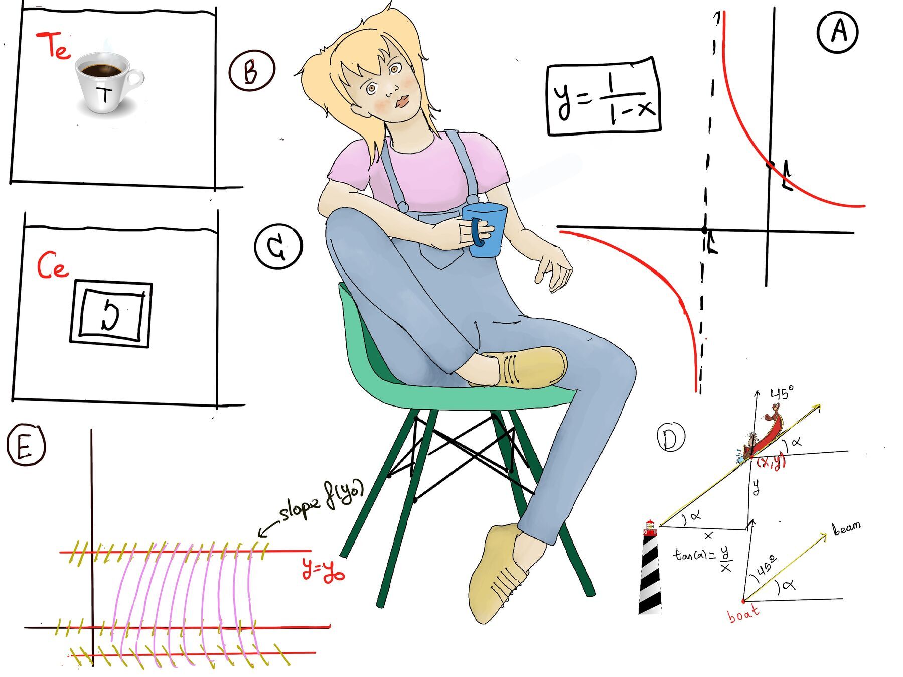
Refer to Figure B for a visual representation of the cooling process and aid in understanding it.

The general solution to Newton’s Law of Cooling $\frac{dT}{dt} = -k(T - T_e)$ is: $\boxed{T = T_e + (T_0-T_e)e^{-kt}}$

1. Insert the known initial conditions. Initial temperature: $T_0 = 180 \deg$ F; ambient temperature: $T_e = 76 \deg$ F. Substitute into the general solution: $T(t) = 76 + (180 - 76)e^{-kt} = 76 + 104e^{-kt}$.
2. Apply the temperature at t = 5 minutes. We are told that T(5) = 168°F, then $ T(t) = 76 +104e^{-5·k} = 168 ↭ 104e^{-5·k} = 168 -76 = 92 ↭ 104e^{-5·k} = 92$
3. Solve for the exponential term: $e^{-5·k}$: $e^{-5·k} = \frac{92}{104} = 0.8846.$
4. Take the natural logarithm of both sides: $-5k = ln(0.8846)$.
5. Solve for k: $k = \frac{-ln(0.8846)}{5}≈ \frac{0.122}{5} ≈ 0.0245$ per minute. The cooling constant k is approximately 0.0244 per minute. This value quantifies the rate at which the coffee cools down in the given environment or moves toward the ambient temperature. A larger 𝑘 would indicate faster cooling; a smaller 𝑘 would indicate slower cooling,

Diffusion Model: Salt Concentration Across a Semi‑Permeable Membrane

Diffusion processes provide another elegant example of first‑order linear differential equations. Just as Newton’s Law of Cooling models how temperature approaches equilibrium, diffusion models describe how concentrations equalize across boundaries.

Consider a chamber containing a salt solution whose internal concentration at time t is C(t). The chamber is immersed in a surrounding water bath with a constant external concentration $C_e$. A semi‑permeable membrane separates the two regions and allows salt to diffuse across it.

The key physical principle is simple: Salt diffuses from regions of higher concentration to regions of lower concentration, and the rate of diffusion is proportional to the concentration difference.

This leads to the differential equation: $\boxed{\frac{dC}{dt} = k(C_e-C)}$ where:

• C(t) is the concentration of salt inside the chamber at time t (internal salt concentration).
• $C_e$ is the constant external concentration of salt in the water bath.
• k is a positive constant representing the diffusion rate.
• $\frac{dC}{dt}$ represents the rate of change of the internal concentration.

This equation is similar to the cooling equation. It states that the rate at which the internal salt concentration changes is proportional to the difference between the external and internal concentrations.

Physical Interpretation of the Differential Equation

This equation mirrors the cooling equation in structure and meaning:

• If $C < C_e$, the internal concentration is lower than the external concentration (the chamber is less salty than the bath), so salt diffuses into the chamber, resulting in a increase in internal concentration $\frac{dC}{dt} > 0$.
• If $C > C_e$, the internal concentration is higher than the external concentration (the chamber is saltier than the bath), so salt diffuses out of the chamber, resulting in a decrease in internal concentration ($\frac{dC}{dt} < 0$). Refer to Figure C for a visual representation and aid in understanding it.
• If $C = C_e$, there is an equilibrium → no net diffusion → $\frac{dC}{dt} = 0$.

Rewriting the equation in standard linear form: $\frac{dC}{dt}+kC = kC_e$. Again, this matches the previously studied standard form y’ + p(t)y = q(t), where y = C(t), p(t) = k, and $q(t) = kC_e$.

Solution Using Integrating Factor

1. Find the integrating factor: $μ(t)=e^{\int p(t)dt} = e^{\int kdt} = e^{kt}$
2. Multiply both sides by the integrating factor: $e^{kt}\frac{dC}{dt} + e^{kt}kC = e^{kt}kC_e ↭ \frac{d}{dt}(e^{kt}C) = e^{kt}kC_e$
3. Integrate both sides: $e^{kt}C = \int e^{kt}kC_edt = C_ee^{kt} ↭ e^{kt}C = C_ee^{kt}+C'$, where C’ is the constant of integration.
4. Solve for C(t): $C = C_e + C'e^{-kt}$.
5. Apply initial conditions. If C(0) = C₀, then $C_0 = C_e + C'e^{-0·t} = C_e + C' ⇒ C' = C_0 - C_e$
6. Final Solution: $\boxed{C(t) = C_e + (C_0 - C_e)e^{-kt}}$.
7. Interpretation of the Solution. The internal concentration C(t) exponentially approaches the external concentration C_e over time. As t → ∞, $e^{-kt}→0, \lim_{t \to \infty} C(t) = C_e$.

Interpretation of the Solution

The factor $e^{-kt}$ represents exponential decay of the concentration difference $C(t) - C_e$. In other words, the internal concentration C(t) exponentially approaches the external concentration $C_e$.

This means:

• The difference between internal and external concentrations shrinks exponentially.
• The system behaves like a first‑order low‑pass filter: it “forgets” its initial concentration at an exponential rate.

Role of the Diffusion Constant k

The rate of diffusion k determines how quickly the internal concentration C(t) approaches the external concentration $C_e$ or how quickly equilibrium is reached:

• Larger k means faster diffusion; the chamber concentration quickly approaches $C_e$.
• Smaller k means slower diffusion; the chamber concentration changes more gradually.

In both applications, the solutions exhibit exponential behavior, reflecting how the quantity of interest approaches equilibrium over time.

Bibliography

1. NPTEL-NOC IITM, Introduction to Galois Theory.
2. Algebra, Second Edition, by Michael Artin.
3. LibreTexts, Calculus and Calculus 3e (Apex). Abstract and Geometric Algebra, Abstract Algebra: Theory and Applications (Judson).
4. Field and Galois Theory, by Patrick Morandi. Springer.
5. Michael Penn, and MathMajor.
6. Contemporary Abstract Algebra, Joseph, A. Gallian.
7. YouTube’s Andrew Misseldine: Calculus. College Algebra and Abstract Algebra.
8. MIT OpenCourseWare [18.03 Differential Equations, Spring 2006], YouTube by MIT OpenCourseWare.
9. Calculus Early Transcendentals: Differential & Multi-Variable Calculus for Social Sciences.