First-order Linear with Constant Coefficients

One who asks a question is a fool for a minute; one who does not remains a fool forever, Chinese proverb

Recall. Algebraic and differential equations.

An algebraic equation is a mathematical statement asserting that two algebraic expressions are equal.. These expressions are constructed using:

1. Dependent and independent variables. Variables are symbols representing unknown quantities. Variables can be:
   Independent Variables: Variables or input that can be chosen (or change) freely.
   Dependent Variables: Variables that depend on the independent variables.
2. Constants. Fixed numerical values that do not change, e.g., 2, π, 7.
3. Algebraic operations. Operations such as addition, subtraction, multiplication, division, exponentiation, powers, and root.

An algebraic equation typically has the following general form: Expression₁ = Expression₂, where the two expressions are set equal to each other.

Examples: y = 2x + 4 (simple linear equation, represents a straight line with a slope of 2 and a y-intercept of 4), ax² + bx + c = 0 (quadratic equation, it represents a parabola), $ln(xy + t) = z·sin(\sqrt{x})$.

Definition. A differential equation is an equation that involves one or more functions and their derivatives. It relates the function itself (the dependent variable), its derivatives with respect to one or more independent variables (rates of change), and the independent variable(s) themselves, e.g., $\frac{dy}{dx} = 3x +5y, y' + y = 4xcos(2x), \frac{dy}{dx} = x^2y+y, etc.$

If an algebraic equation is a “snapshot” of a relationship, a differential equation is the “instruction manual” for how that relationship moves and changes.

Key Components (e.g., $\frac{dy}{dx} = 3x +5y$):

• Dependent variables: The function y (or y(x)) we are trying to find or solve for. Variable(s) (y) that depend on one or more other variables.
• Independent variables: Variable(s) (x) upon which the dependent variables depend and we differentiate with respect to (often time or space).
• Derivatives: Expressions like $\frac{dy}{dx}$ or y’ that represent the rate at which the dependent variable (y) change with respect to the independent variable (x).

First-Order Linear Ordinary Differential Equations (ODEs)

First-order linear differential equations are fundamental tools in mathematical modeling across various disciplines, including physics, engineering, biology, and economics. They are used to describe dynamic systems where the rate of change of a quantity depends linearly on the quantity itself and, frequently, on external inputs.

Definition. A first-order linear ordinary differential equation is an ordinary differential equation (ODE) involving an unknown function y(x), its first derivative y′, and functions of the independent variable x, which can be written in the general form:: a(x)y' + b(x)y = c(x) where:

• y = y(x) is the unknown function of the independent variable x.
• y′ = $\frac{dy}{dx}$ is the first derivative of y with respect to x.
• a(x), b(x), and c(x) are known continuous functions of x.

These equations are termed “linear” because the unknown function y and its derivative y’ strictly appear to the first power. They are never multiplied together, squared, or composed inside nonlinear functions (like sin(y) or $e^y$).

If the forcing function c(x) = 0 for all x in the interval of interest, the equation simplifies to: a(x)y’ + b(x)y = 0. Such an equation is called a homogeneous linear differential equation. If $c(x) \ne 0$, it is non-homogeneous.

The Standard Linear Form

To standardize the equation and prepare it for universal solution methods, we divide both sides of the general form by a(x), assuming a(x) ≠ 0: y’ + p(x)y = q(x) where $p(x)=\frac{b(x)}{a(x)}\text{ and }q(x) = \frac{c(x)}{a(x)}$ This is the standard linear form of a first-order differential equation, which is more convenient for applying solution methods, such as the integrating factor method.

Solving the Equation Using Integrating Factors

The integrating factor method is a brilliant and highly effective algebraic technique. It involves multiplying the entire standard-form equation by a carefully crafted mathematical function—the integrating factor—which compresses the left side of the equation into a single, easily integrable derivative via the product rule.

Here are the step-by-step mechanics:

1. Write in Standard Form. Ensure the equation is arranged as $\frac{dy}{dx} +p(x)y = q(x)$
2. Calculate the integrating Factor μ(x). The integrating factor μ(x) is defined as the exponential of the integral of p(x): $μ(x)=e^{\int p(x)dx}$. This function is chosen so that when we multiply both sides of the differential equation by μ(x), the left-hand side becomes the derivative of μ(x)y.
   

   Note: We typically ignore the constant of integration +C during this specific step, as any constant multiplier will eventually cancel out.

3. Multiply Both Sides of the equation by the Integrating Factor: $μ(x)\frac{dy}{dx} +μ(x)p(x)y = μ(x)q(x)$.
4. Collapse the Left-Hand Side: By design, the left side is now the exact expansion of the derivative of the product μ(x)y. We can rewrite the equation as: $\frac{d}{dx}[μ(x)y] = μ(x)q(x)$
5. Integrate both sides with respect to x: $\int \frac{d}{dx}[μ(x)y]dx = \int μ(x)q(x)dx \iff μ(x)y = \int μ(x)q(x)dx + C$.
6. Solve for y(x). Divide by μ(x) to isolate the unknown function: $y(x) = \frac{1}{μ(x)}(\int μ(x)q(x)dx + C)$

Equations with Constant Coefficients

When p(x) and q(x) are constants, the equation simplifies dramatically, and finding the solutions become more straightforward. This is the most common form encountered in introductory physics and engineering circuits.

Standard Form with Constant Coefficients

Consider the equation modeled over time t: $\frac{dy}{dt} + ky = q(t)$ where:

• k is a constant positive coefficient, k > 0.
• q(t) is a given input or forcing function of t.

Applying the Integrating Factor Method

1. Identify p(t) and q(t): p(t) = k (constant), and q(t) is the given function of t.
2. Calculate the Integrating Factor μ(t). The integrating factor is: $μ(t) = e^{\int p(t)dt} = e^{\int kdt} = e^{kt}$
3. Multiply Both Sides by μ(t): $e^{kt}\frac{dy}{dt} + ke^{kt}y = e^{kt}q(t)$.
4. Simplify the Left-Hand Side: $e^{kt}\frac{dy}{dt} + ke^{kt}y = \frac{d}{dt}(e^{kt}·y)$. So the equation becomes: $\frac{d}{dt}(e^{kt}·y) = e^{kt}q(t)$
5. Integrate Both Sides: $\int \frac{d}{dt}(e^{kt}·y)dt = \int e^{kt}q(t)dt ↭ e^{kt}·y = \int e^{kt}q(t)dt + C$
6. Solve for y: $y(t) = \frac{1}{μ(t)}(\int μ(t)q(t)dt + C)$. Therefore, $\boxed{y(t) = e^{-kt}(\int e^{kt}q(t)dt + C)}$

Interpretation of the Solution

The total solution y(t) naturally splits into two distinct behavioral components: $\boxed{y(t) = y_{part}(t) + y_{hom}(t)}$.

• Particular Solution (Forced / Steady-State Response). The first term $y_{part}(t) = e^{-kt}\int q(t)e^{kt}dt$ is the forced response driven entirely by the external input q(t). If k > 0, the initial transient effects will eventually die out, and this term will completely dominate the behavior of y(t) as t → ∞. In other words, it represents the part of the solution that persists over time (how the system responds in the long term). For this reason, it is frequently referred to as the steady-state solution (Refer to Figure v for a visual representation).
• Homogeneous Solution (Natural / Transient Response). The second term $y_{hom}(t)=Ce^{-kt}$ is the transient solution (also called the natural response). It relies heavily on the constant C, which is determined by the system’s initial conditions. Because k > 0, this term decays exponentially to zero as t→∞. It represents a temporary phase of adjustment that fades away over time.

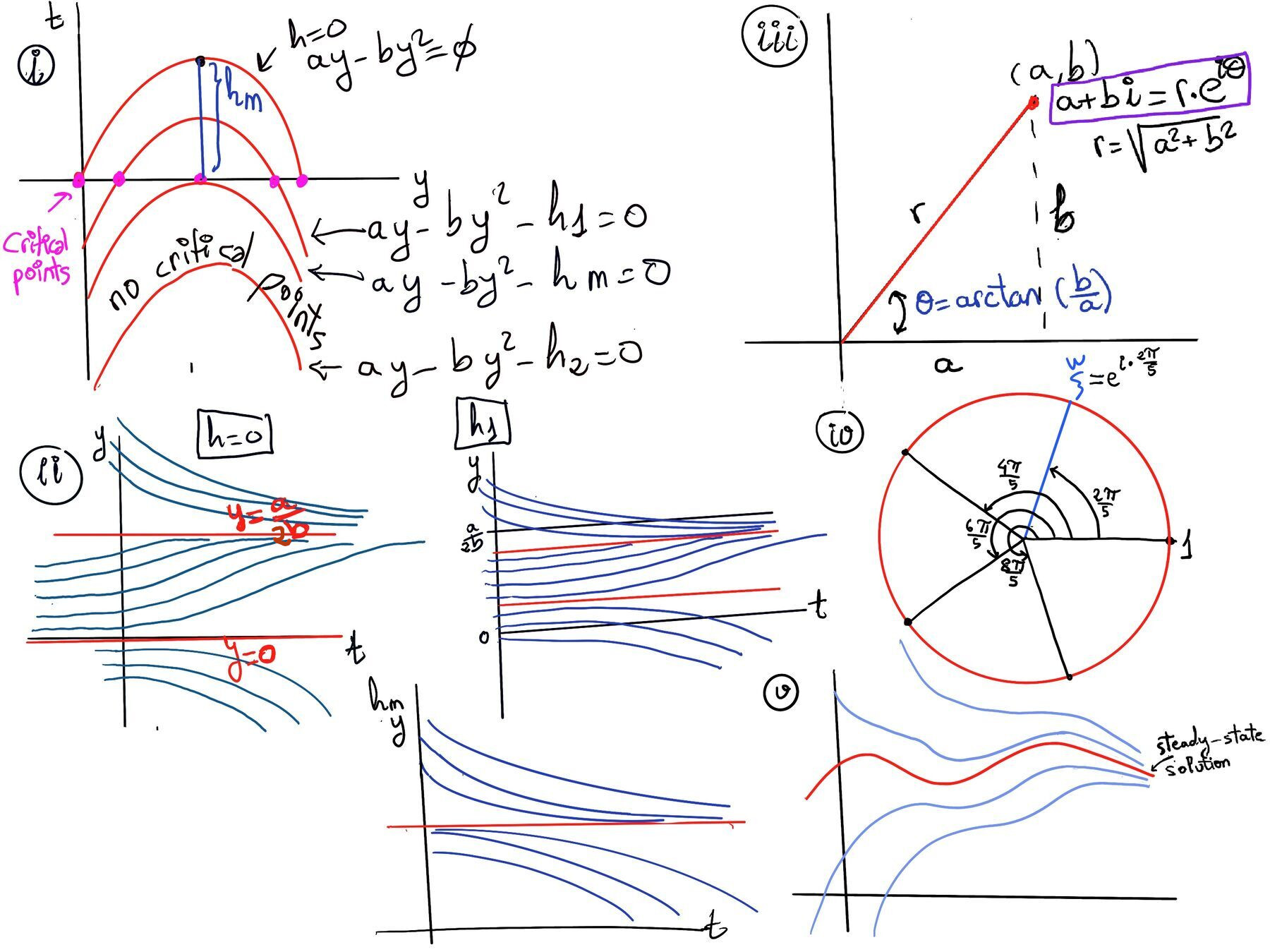
Sometimes the equation y’ + ky = kq_e(t) is expressed as $\frac{1}{k}y' + y = q_e(t)$ where q_e(t) is called the input.

Example: Solving a First-Order Linear ODE with Constant Coefficients

Let’s walk through a concrete example of solving a non-homogeneous first-order linear differential equation using the integrating factor method.

Consider the following differential equation: $\frac{dy}{dt}+2y = e^{-2t}$.

Step-by-Step Solution

1. Identify p(t) and q(t) in the Standard form. The equation is already written in the standard form $\frac{dy}{dt} +p(t)y = q(t)$. From inspection, we can extract: p(t) = 2, $q(t) = e^{-2t}$.
2. Calculate the integrating Factor μ(t): $μ(t)=e^{\int p(t)dt} = e^{\int 2dt} = e^{2t}$
3. Multiply Both Sides by the Integrating Factor. Multiplying every term in the original ODE by $e^{2t}$ gives: $e^{2t}\frac{dy}{dt}+2e^{2t}y = e^{2t}e^{-2t} = 1 ⇒[\text{Since } e^{2t}e^{-2t} = 1 \text{, the right-hand side simplifies beautifully:}] e^{2t}\frac{dy}{dt}+2e^{2t}y =1$.
4. Recognize the Left-Hand Side as a Derivative. By design, the left side of the equation matches the expanded form of the product rule derivative $\frac{d}{dt}[\mu(t)\cdot y]$. We can condense it down to: $\frac{d}{dt}[e^{2t}y] = 1$
5. Integrate both sides: $\int \frac{d}{dt}[e^{2t}y]dt = \int 1dt ↭ e^{2t}y = t + C$.
6. Solve for y(t). Isolate y(t) by multiplying the entire equation by $ e^{-2t}$: $\boxed{y(t) = e^{-2t}(t + C)}$

Interpretation of the solution

The general solution is mathematically composed of two distinct responses: $y(t) = y_{\text{particular}(t)} + y_{\text{homogeneous}(t)}$

• The Homogeneous Response / Transient Solution is $y_{\text{homogeneous}(t)} = Ce^{-2t}$, which decays exponentially to zero as t → ∞. This represents the system’s natural response dictates strictly by its initial state. The constant C is determined entirely by the initial value $y(0) = y_0. y(0) = 0 \cdot e^0 + C \cdot e^0 \implies C = y_0$.
• The Particular Solution / Forced Response is $y_{\text{homogeneous}(t)} te^{-2t}$. This represents the system’s response to the specific external input forcing function $q(t) = e^{-2t}$. Because the external forcing function $q(t) = e^{-2t}$ itself decays to zero, the force response $te^{-2t}$ also eventually vanishes as $t \to \infty$.

Thus, the final explicit solution matching the initial condition is: $y(t) = e^{-2t}(t + y_0)$

In this specific example, the entire solution diminishes over time and converges back to absolute rest (y = 0).

Physical Interpretation: The system returns to equilibrium over time. Any initial perturbations (captured by C) decay exponentially.

The Superposition Principle

The superposition principle is a fundamental structural pillar of linear systems, particularly in the study of linear differential equations. It allows us to break up a problem into simpler, more manageable parts, and then at the end assemble the answer from its simpler pieces. This principle is immensely powerful because it leverages the linearity property of differential equations.

It states that if a system is driven by multiple independent inputs, you can break the problem up into simpler parts, solve for each input individually, and then add the individual answers together to find the total response.

Let’s consider the first-order linear differential equation: y’ + p(t)y = q(t) where:

• y(t) is the unknown state response of the system we aim to solve for.
• p(t) is a known function representing the internal parameters of the system.
• q(t) is a known function representing the external input or forcing function.

In this context, we can think of the left-hand side $\frac{dy}{dt}+p(t)y$ as representing the system (the physical “system rules”) and the right-hand side q(t) as the input to the system.

For any given input q(t) that yields an output or solution y(t), we can write this relationship as $q(t) \implies y(t)$ (read input q leads to output y).

The Superposition Principle Explained

The superposition principle states that in a linear system, the response (output) to a weighted sum of inputs (e.g., $q_1(t)$ and $q_2(t)$) is equal to the exact same weighted sum of their individual responses (responses to each input individually).

Mathematically, if $q_1(t)$ leads to solution $y_1$ ($q_1 \implies y_1$) and $q_2(t)$ leads to solution $y_2$ ($q_2 \implies y_2$), then the combined input $c_1q_1(t) + c_2q_2(t)$ leads directly to the solution: $c_1y_1(t) + c_2y_2(t)$ ($c_1q_1 + c_2y_2 \implies c_1y_1 + c_2y_2$). This principle holds because the differential equation is linear and linear systems allow for the sum of solutions to be a solution itself.

Proof:

Because calculus derivatives are linear operators, proving this requires only a few straightforward algebraic steps. Let’s plug the proposed combined solution $y(t) = c_1y_1(t) + c_2y_2(t)$ into the left-hand side of our differential equation: $\frac{d(c_1y_1 + c_2y_2)}{dt} + p(c_1y_1 + c_2y_2)$

Distribute the derivative operator and the coefficient function p(t): $c_1\frac{dy_1}{dt} + c_2\frac{dy_2}{dt} + c_1py_1 + c_2py_2$.

Group the terms by their respective scaling constants $c_1$ and $c_2$: $c_1(\frac{dy_1}{dt} + py_1) + c_2(\frac{dy_2}{dt} + py_2)$

Since we already know that $y_1$ solves the equation for $q_1$ and $y_2$ solves it for $q_2$ ($q_1 \implies y_1, q_2 \implies y_2$), we get: $c_1q_1 + c_2q_2.$

The left side simplifies perfectly into the combined input. Therefore, the combined output $y(t) = c_1y_1(t) + c_2y_2(t)$ is mathematically guaranteed to be the exact solution to the differential equation under the combined input $q(t) = c_1q_1(t) + c_2q_2(t)$.

Example Using Superposition

Let’s look at a practical example that demonstrates how to use the superposition principle to solve a more complex first-order linear ordinary differential equation by breaking it down into simpler, modular parts.

• Solve the differential equation: $\frac{dx}{dt} + 2x = 2 + 3e^{-2t}$

Step 1: Decompose the Input Forcing Function. We can break this problem into two simpler differential equations. The right-hand side input, $q(t) = 2 + 3e^{-2t}$ can be viewed as a linear combination of two fundamental baseline signals. Baseline Input 1, $q_1(t) = 1$. Baseline Input 2, $q_2(t) = e^{-2t}$. Therefore, the total input is a scaled combination of these two inputs: $q(t) = 2q_1(t) + 3q_2(t).$

According to the Superposition Principle, if we find the individual responses $x_1(t)$ and $x_2(t)$ to these baseline inputs, our total solution will simply be: $x(t) = 2x_1(t) + 3x_2(t)$.

Step 2: Solve Each Subproblem Individually

Equation 1. $\frac{dx_1}{dt} + 2x_1 = 1$. The solution can be found:

1. Calculate the integrating factor: $μ(t)=e^{\int p(t)dt} = e^{\int 2dt} = e^{2t}$.
2. Multiply Both Sides by the Integrating Factor: $e^{2t}\frac{dx_1}{dt} + 2x_1e^{2t} = e^{2t}$.
3. Recognize the Left-Hand Side as a Derivative: $\frac{d}{dt}[e^{2t}x_1] = e^{2t}$.
4. Integrate both sides: $\int \frac{d}{dt}[e^{2t}x_1]dt = \int e^{2t}dt↭e^{2t}x_1 = \frac{e^{2t}}{2} + C_1$.
5. Solve for x: $x_1(t) = \frac{1}{2} + C_1e^{-2t}$ (i)

Equation 2. $\frac{dx_2}{dt}+2x_2 = e^{-2t}$,

1. Calculate the integrating factor: $μ(t)=e^{\int p(t)dt} = e^{\int 2dt} = e^{2t}$.
2. Multiply Both Sides by the Integrating Factor: $e^{2t}\frac{dx_2}{dt} + 2x_2e^{2t} = e^{2t}e^{-2t} = 1$.
3. Recognize the Left-Hand Side as a Derivative: $\frac{d}{dt}[e^{2t}x_2] = 1$.
4. Integrate both sides: $\int \frac{d}{dt}[e^{2t}x_2]dt = \int dt↭e^{2t}x_2 = t + C_2$.
5. Solve for x: $x_2(t) = e^{-2t}(t+C_2)$ (ii)

Step 3: Combine Solutions Using Superposition. Now, we construct the final composite solution x(t) by scaling and adding our two individual subproblem solutions together: $x(t) = 2x_1(t) + 3x_2(t) = 2(\frac{1}{2} + C_1e^{-2t}) + 3e^{-2t}(t+C_2) = 1 + 2C_1e^{-2t} + 3e^{-2t}t + 3e^{-2t}C_2 =[\text{Simplify}] 1 + e^{-2t}(3t + 2C_1 + 3C_2) = 1 + e^{-2t}(3t + C)$.

This gives us our final general explicit solution: $\boxed{x(t) = 1 + e^{-2t}(3t + C)}$ where C is a single consolidated arbitrary constant defined as $C = 2C_1 + 3C_2$.

Step 4: Physical & Mathematical Interpretation.

• The Constant Steady-State Response. The standalone constant term 1 is the steady-state solution generated exclusively by the continuous driving input of 2.
• The second term $e^{-2t}(3t + C)$ is the transient response, an internal mix of the forced response from the decaying exponential input $3e^{-2t}$ and the system’s own natural response to its initial state (C).

Long-Term System Behavior (t → ∞). What happens to the system in the long run? We evaluate the limit as time goes to infinity:

$\lim_{t \to \infty}x(t) = \lim_{t \to \infty} [1 + \frac{3t + C}{e^{2t}}]$

Using L’Hôpital’s Rule on the fraction, $\lim_{t \to \infty} \frac{3}{2e^{2t}} = 0.$ Because exponential growth in the denominator dramatically outpaces the linear growth in the numerator, the entire transient term exponentially decays to zero.

Therefore, $\lim_{t \to \infty}x(t) = 1$.

No matter what the initial conditions or transient inputs are, the system naturally clears out its temporary behaviors and smoothly settles down to a stable operating state of x = 1.

Bibliography

1. NPTEL-NOC IITM, Introduction to Galois Theory.
2. Algebra, Second Edition, by Michael Artin.
3. LibreTexts, Calculus and Calculus 3e (Apex). Abstract and Geometric Algebra, Abstract Algebra: Theory and Applications (Judson).
4. Field and Galois Theory, by Patrick Morandi. Springer.
5. Michael Penn, and MathMajor.
6. Contemporary Abstract Algebra, Joseph, A. Gallian.
7. YouTube’s Andrew Misseldine: Calculus. College Algebra and Abstract Algebra.
8. MIT OpenCourseWare [18.03 Differential Equations, Spring 2006], YouTube by MIT OpenCourseWare.
9. Calculus Early Transcendentals: Differential & Multi-Variable Calculus for Social Sciences.