First-Order Autonomous ODEs II. The Logistic Equation & Harvesting

Irony is wasted on the stupid, Oscar Wilde

To err is human, to blame it on someone else is even more human, Jacob’s Law

Recall. Algebraic and differential equations.

An algebraic equation is a mathematical statement asserting that two algebraic expressions are equal.. These expressions are constructed using:

1. Dependent and independent variables. Variables are symbols representing unknown quantities. Variables can be:
   Independent Variables: Variables or input that can be chosen (or change) freely.
   Dependent Variables: Variables that depend on the independent variables.
2. Constants. Fixed numerical values that do not change, e.g., 2, π, 7.
3. Algebraic operations. Operations such as addition, subtraction, multiplication, division, exponentiation, powers, and root.

An algebraic equation typically has the following general form: Expression₁ = Expression₂, where the two expressions are set equal to each other.

Examples: y = 2x + 4 (simple linear equation, represents a straight line with a slope of 2 and a y-intercept of 4), ax² + bx + c = 0 (quadratic equation, it represents a parabola), $ln(xy + t) = z·sin(\sqrt{x})$.

Definition. A differential equation is an equation that involves one or more functions and their derivatives. It relates the function itself (the dependent variable), its derivatives with respect to one or more independent variables (rates of change), and the independent variable(s) themselves, e.g., $\frac{dy}{dx} = 3x +5y, y' + y = 4xcos(2x), \frac{dy}{dx} = x^2y+y, etc.$

If an algebraic equation is a “snapshot” of a relationship, a differential equation is the “instruction manual” for how that relationship moves and changes.

Key Components (e.g., $\frac{dy}{dx} = 3x +5y$):

• Dependent variables: The function y (or y(x)) we are trying to find or solve for. Variable(s) (y) that depend on one or more other variables.
• Independent variables: Variable(s) (x) upon which the dependent variables depend and we differentiate with respect to (often time or space).
• Derivatives: Expressions like $\frac{dy}{dx}$ or y’ that represent the rate at which the dependent variable (y) change with respect to the independent variable (x).

Existence and Uniqueness Theorem

The Existence and Uniqueness Theorem provides crucial insight into the behavior of solutions to first-order differential equations ODEs. It answers two fundamental questions: Is there a solution? and Is it the only one? It states that if:

• The function $f(x, y)$ (the right-hand side of the ODE when written as $y' = f(x, y)$) is continuous in some neighborhood around a specific point $(x_0, y_0)$ and
• Its partial derivative with respect to y, denoted as $\frac{\partial f}{\partial y}$, is also continuous near $(x_0, y_0)$.

Then, the differential equation y' = f(x, y) has a unique solution to the initial value problem through the point (x₀, y₀), meaning that it perfectly satisfies the initial condition $y(x_0) = y_0$.

This theorem is a mathematician’s safety net: it ensures that under these well-behaved conditions, a solution definitively exists and is absolutely unique near $x = x_0$. The physical system modeled by the ODE will only follow one distinct path.

The Logistic Equation

The Basic Exponential Growth Model

The simplest mathematical model of population growth is described by the linear differential equation: $\frac{dy}{dt} = ky$ where:

• y(t) represents the population at time k,
• k is the intrinsic growth rate (a positive constant).

This equation states that the rate of change of a given population is stricly proportional to the population size itself. As the population increases, the rate of growth also increases exponentially. The solution to this equation is $y(t) = y_0e^{kt}$ where $y_0$ is the initial population at time t = 0.

Limitation of the Exponential Model

While this model successfully captures the essence of unchecked population growth (like bacteria in a freshly prepared petri dish), it is overly simplistic and unrealistic for long-term modeling. It fails to account for environmental limitations and Earth’s limited resources, which are crucial in real-world scenarios. In reality, resources such as food scarcity, physical space, and predation inevitably limit population growth.

Two things are infinite: the universe and human stupidity; and I’m not sure about the universe, Albert Einstein.

This quote humorously highlights the absurdity of assuming infinite resources, which is the underlying assumption required for indefinite exponential growth.

The Logistic Growth Model

To address the severe limitations of the exponential model, the logistic growth model introduces the concept of a carrying capacity. Logistic growth introduces the idea that as a population increases and resources become scarce, the net growth rate must decrease. The logistic equation accounts for limited resources by incorporating a subtraction term that artificially slows the growth rate as the population size grows.

The logistic equation models population growth with a carrying capacity, accounting for limited resources. The logistic differential equation is given by: $\frac{dy}{dt} = ay -by^2$ where:

• y(t) represents the population at time t.
• a is the intrinsic growth rate (the rate at which the population would grow without any limitations or infinite resources),
• b is a positive constant representing how the population growth is limited by limited resources.

Interpretation of terms:

• The term ay represents the natural exponential growth of the population, proportional to its current size.
• The term $-by^2$ represents the limitation imposed by finite resources (such as food, space, competition, environmental issues, disease, etc.). As the population grows larger, this term $-by^2$ grows massively, eventually overwhelming the $ay$ term and slowing the rate of growth until the population reaches a stable size.

The logistic model is also used in modeling the spread of diseases (epidemiology), the adoption of new technologies, and other phenomena exhibiting saturation behavior.

Qualitative Analysis of the Logistic Differential Equation

1. Autonomous Nature. The logistic equation is an autonomous differential equation because the rate of change $\frac{dy}{dt}$ ​depends only on the dependent variable y and not explicitly on the independent variable t. Autonomous ODEs allow us to use qualitative techniques (like phase lines) to completely understand the behavior of solutions without having to integrate them.

   Solutions to autonomous equations are invariant under time translation, meaning the “rules of growth” depend only on the current population size $y$, not on the current year $t$.

2. Finding Critical Points (Equilibrium Solutions). Critical points occur where the rate of change of the population halts: $\frac{dy}{dt} = ay -by^2 = 0↭[\text{Factor out y}] y(a -by) = 0$. This gives two roots: $y = 0 \quad \text{and} \quad y = \frac{a}{b}$.
   At these critical points, the population remains completely constant (Refer to Figure 3 for a visual representation and aid in understanding it). 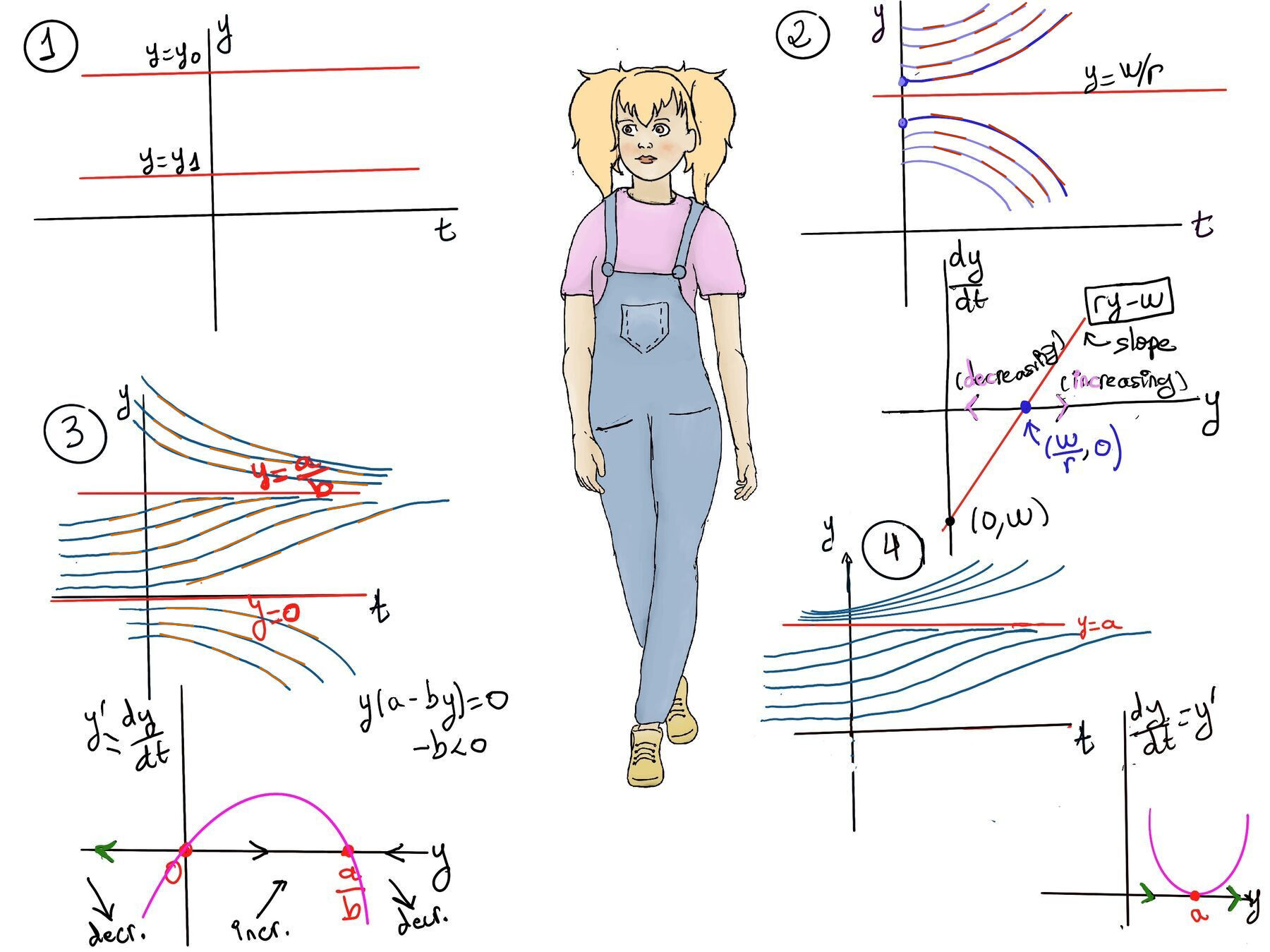$\star$: y = 0 represents an unstable critical point, meaning if the population is very small, it is likely to grow. However, if the population reaches zero, it stays at zero (extinction of the population).
   $\star$: y = a/b is a stable critical point, meaning the population naturally gravitates toward and stabilizes at this value. This ratio is called the carrying capacity of the population (often denoted as $L$) — essentially the maximum population that the environment can sustain given its limited resources.

1. Behaviour of the solution. Stability of Critical Points
   The graph of $\frac{dy}{dt} = ay-by^2$ versus y is a downward-opening parabola with roots at y = 0 and $\frac{a}{b}$. The absolute maximum growth rate occurs at the vertex of the parabola, $y = \frac{a}{2b}$ (exactly half the carrying capacity).
   By looking at where the parabola is above or below the axis, we can determine the direction of the population:
   $\star$: If $y > \frac{a}{b}$ or y < 0, the term y(a -by) = 0 becomes negative, making $\frac{dy}{dt} < 0$. The solution is decreasing, which means the population decreases over time. This suggests that if the population exceeds the environment's carrying capacity, starvation or disease will cause it to shrink back down due to resource constraints. Besides, populations that start with negative values (negative population sizes are not biologically meaningful but can be considered mathematically) will move further away from y = 0.
   $\star$: If $0 < y < \frac{a}{b}$, the function y(a -by) = 0 is positive, making $\frac{dy}{dt} > 0$. The solution is increasing, which means the population thrives and grows toward the stable carrying capacity a/b.
   Basically, we can observe arrows pointing away from y = 0 (unstable equilibrium) and toward y = L (stable equilibrium). Curves starting above L decrease toward L. Curves starting below L and above 0 increase toward L.
   The general behavior is that populations starting below the carrying capacity grow upwards and populations starting above the carrying capacity shrink downwards, both inevitably converge on the stable equilibrium $y = \frac{a}{b}$.

Solving the Logistic Differential Equation Explicitly

To find the exact formula for the population $y(t)$ at any given time, we use separation of variables.

1. Separate Variables:
   $\frac{dy}{dt} = ay -by^2 ↭[\text{Factor out y}] \frac{dy}{dt} = y(a-by) ↭ [\text{Separable variables}] \frac{dy}{y(a-by)} = dt$.

2. Partial Fraction Decomposition: $\frac{1}{y(a-by)} = \frac{A}{y} + \frac{B}{a-by}$
   Multiply both sides by by the denominator y(a−by): $1 = A(a-by)+By$. Set up equations to solve for A and B:
   $\begin{cases} -Ab + B = 0~\text{. Coefficient of y (i)} \\\ Aa = 1 ~\text{. Constant term (ii)}\end{cases}$
   (ii) ⇒ $A = \frac{1}{a}$. (i)⇒ $B = Ab = \frac{b}{a}$, hence $\frac{1}{y(a-by)} = \frac{1}{a}\frac{1}{y} + \frac{b}{a}\frac{1}{a-by}$

3. Integrate Both Sides: $\int (\frac{1}{a}\frac{1}{y} + \frac{b}{a}\frac{1}{a-by})dy = \int dt$
   $\int \frac{1}{a-by}dy =$[Let t = a-by, dt = -bdy] $\frac{-1}{b}\int \frac{1}{t}dt = \frac{-1}{b}ln|t| = \frac{-1}{b}ln|a-by|$

4. Combine both integral and simplify the expression: $\frac{1}{a}ln|y| + \frac{b}{a}·\frac{-1}{b}ln|a-by| = t + C ↭ \frac{1}{a}ln|y| + \frac{-1}{a}ln|a-by| = t + C.$ Multiply both sides by a to eliminate the fractions: $ln|y|-ln|a-by| = a(t+C)$.
   Assuming the population is between 0 and the carrying capacity, we can drop the absolute values and combine the logarithms: $ln(y)-ln(a-by) = a(t+C)$.
   Combine Logarithms: $ln(\frac{y}{a-by})=a(t+C)↭[\text{Exponentiate both sides}] \frac{y}{a-by} = Ae^{at}$, where A = $e^{aC}$ (absorbing the constant).

5. Solve for y: $\frac{y}{a-by} = Ae^{at} ↭ y = Ae^{at}(a-by)↭[\text{Distribute to the right}] y = aAe^{at} -bAe^{at}y$
   Bring terms involving y to one side: $y + bAe^{at}y = aAe^{at} ↭[\text{Factor out y}] y(1+bAe^{at}) = aAe^{at} ↭ [\text{Solve for y}] y = \frac{aAe^{at}}{1+bAe^{at}}.$
   Divide the numerator and denominator by $A e^{at}$ to clean up the expression: $y = \frac{aA}{e^{-at}+bA}$

6. Apply Initial Conditions.
   Let the population at $t=0$ be $y_0$: $y_0=\frac{aA}{e^{-a·0}+bA} = \frac{aA}{1+bA} \implies y_0(1+bA) = aA ⇒ y_0+y_0bA = aA ⇒y_0 = A(a-by_0)⇒ A = \frac{y_0}{a-by_0}$

7. Final Explicit Solution. Substitute A back into the expression for y(t): $y(t)=\frac{a(\frac{y_0}{a-by_0})}{e^{-at}+b(\frac{y_0}{a-by_0})} = \frac{(\frac{ay_0}{a-by_0})}{(\frac{e^{-at}(a-by_0)+by_0}{a-by_0})} = \frac{ay_0}{e^{-at}(a-by_0)+by_0} = \frac{ay_0e^{at}}{a-by_0 +by_0e^{at}}$.
   $y = \boxed{\frac{ay_0e^{at}}{a+by_0(e^{at}-1)}}$

8. Interpretation of the Solution.
   Let’s see what happens to the math as time goes to infinity.
   $\lim_{t \to \infty} \frac{ay_0e^{at}}{a+by_0(e^{at}-1)} = \frac{a}{b}$ (the leading terms in numerator and denominator are ay₀e^at and by₀e^at) respectively. The math perfectly confirms our qualitative phase line analysis. The population y(t) approaches the carrying capacity y = ^a⁄_b as $t \to \infty$, regardless of the initial population y₀, provided y₀ > 0 (no extinction, population is always positive; by assumption a and b are positive, too).

Therefore,

• If y₀ < ^a⁄_b: The population increases over time, approaching the carrying capacity from below.
• If y₀ > ^a⁄_b: The population decreases over time, approaching the carrying capacity from above.
• If y₀ = 0: The population remains at zero (extinction).

Logistic equation with harvesting

In real-world scenarios, populations may be subject to harvesting, where a portion of the population is removed at a constant rate. This situation commonly arises in fisheries, wildlife management, and forestry, where resource managers attempt to balance human consumption with ecological sustainability.

Mathematical Modeling

The logistic equation with harvesting modifies the original equation to account for this constant removal rate. The equation becomes: $\frac{dy}{dt} = ay -by^2 -h$ where:

• y(t) represents the population at time t.
• a is the intrinsic growth rate (the rate at which the population would grow exponentially without any environmental limitations).
• b is a positive constant representing how density-dependent factors (like food or space constraints) limit the population.
• h is the harvest rate, representing the number of individuals removed from the population per unit time (assumed to be a positive constant, refer to Figure i, ii for a visual representation and aid in understanding it).

Analysis of the Logistic Equation with Harvesting

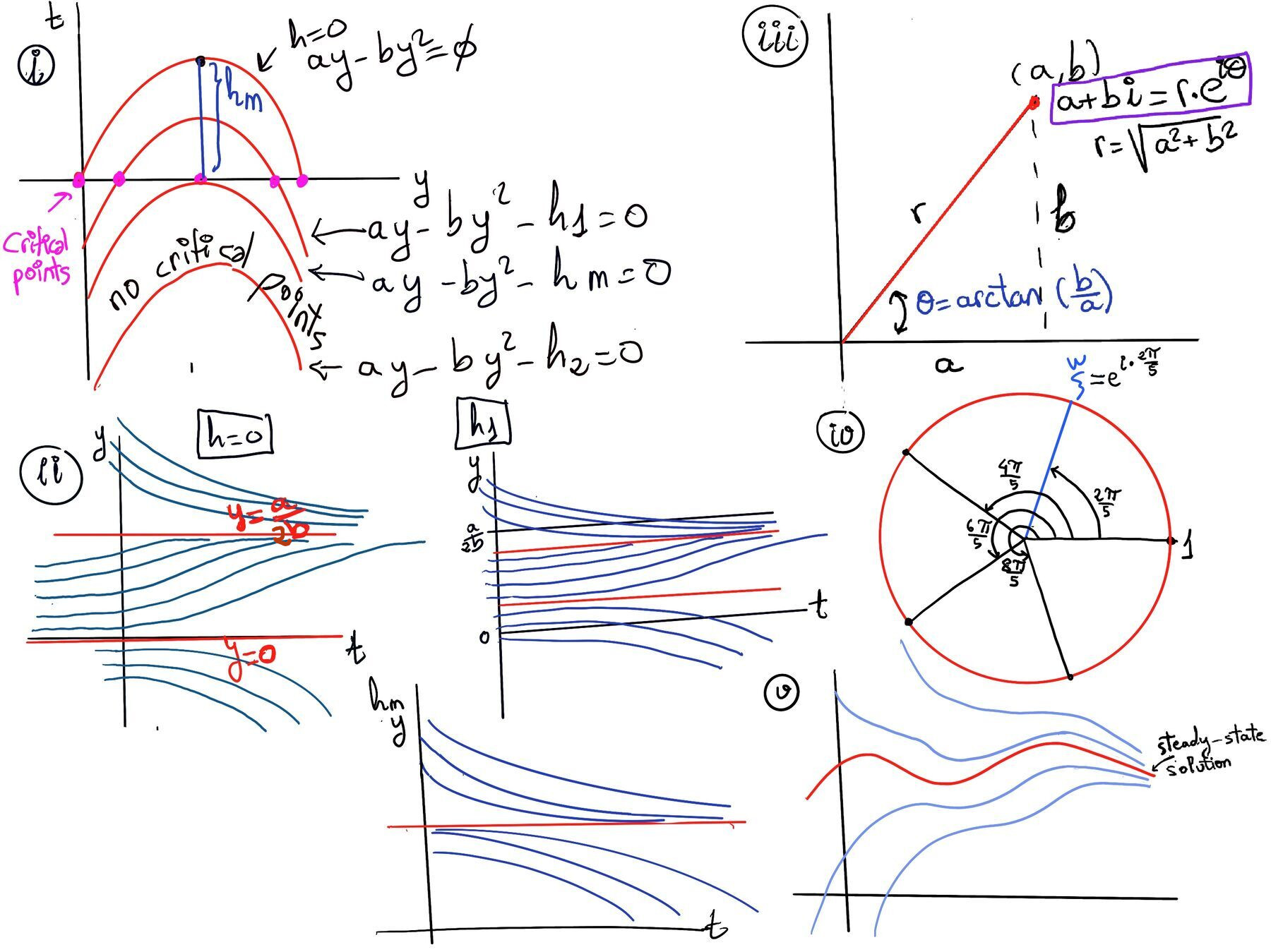
To understand how harvesting affects population dynamics, we must identify the critical points (equilibrium solutions) of this autonomous ODE and evaluate their stability.

1. Case when h = 0. When there is no harvesting, the equation reduces back to the standard logistic equation: $\frac{dy}{dt} = ay-by^2$. As established previously, this system yields an unstable equilibrium at y = 0 and a stable equilibrium at the environmental carrying capacity: $y = \frac{a}{b}$.
2. Case when h > 0. Introducing a constant harvest rate shifts the growth parabola downward. To find the new equilibrium points, we set the growth rate to zero and solve the resulting quadratic equation: $ay -by^2 -h = 0 \implies by^2 -ay + h = 0$.

Applying the quadratic formula yields the equilibrium populations: $y = \frac{a ± \sqrt{a^2-4bh}}{2b}$.

The behavior of the population depends entirely on the value of the algebraic discriminant, $D = a^2-4bh$

Deep-Dive Analysis of the Three Discriminant Conditions:

• Case 1. Sustainable Harvesting. $D = a^2-4bh > 0 \text{ i.e., } h = h_1 < h_m =\frac{a^2}{4b}$. When the harvest rate is strictly below the critical threshold $h_m =\frac{a^2}{4b}$, the equation yields two distinct, real, and positive equilibrium points: $y_1 = \frac{a - \sqrt{a^2-4bh}}{2b}, y_2 = \frac{a + \sqrt{a^2-4bh}}{2b}$ where $y_1$ is the lower equilibrium point and $y_2$ is the higher equilibrium point. Both equilibrium points are positive and meaningful in a biological context.

Both points are biologically meaningful and lie between 0 and the original carrying capacity $\frac{a}{b}$

(1) If $y \lt y_1$ (unstable equilibrium point), the harvest rate outpaces the population’s reproductive capacity $\frac{dy}{dt} < 0$. The population steadily decreases and declines toward total extinction. Thus, $y_1$ acts as an unstable threshold or an “Allee effect” boundary.

The Allee effect is an ecological phenomenon where a population’s individual fitness and growth rate decrease as the population size or density becomes too small

(2) If $y_1 \lt y \lt y_2, \frac{dy}{dt} > 0$. The population growth rate exceeds the harvest rate $\frac{dy}{dt} < 0$. The population increases and grows toward the stable upper equilibrium.

(3) If $y \gt y_2$. Environmental constraints and harvesting combined cause the population to decline $\frac{dy}{dt} < 0$, the population decreases back toward $y_2$. Consequently, if the initial population begins safely above the threshold $y_1$, the population can successfully sustain itself and stabilize at $y_2$.

Conclusion: Harvesting is sustainable as long as the rate (h) is below $h_m =\frac{a^2}{4b}$

• Case 2. The Critical Threshold. When the harvest rate matches the maximum sustainable yield (the discriminant becomes zero, $D = a^2-4bh = 0 \iff h = h_m = \frac{a^2}{4b}$), there is a single, real, repeated root y = $\frac{a}{2b}$. Because the growth parabola has been shifted down by exactly $h = h_m$, its vertex rest precisely on the horizontal axis, f(y) = $-b(y - \frac{a}{2b})^2$.

Because the squared term is always positive or zero, f(y) ≤ 0 for all real values of y. Let’s examine the behavior around this point:

(1) If $y \gt \frac{a}{2b}, \frac{dy}{dt} \lt 0$, meaning the population decreases toward $\frac{a}{2b}$.

(2) If $y \lt \frac{a}{2b}, \frac{dy}{dt} \gt 0$, meaning the population continues to decrease away from $\frac{a}{2b}$ toward extinction.

Because solutions approach it from above but flee from it below, this single critical point is truly semi-stable (precarious equilibrium). This creates a precarious ecological cliff. Any minor environmental fluctuation or slight over-harvesting that pushes the population even a fraction below y = $\frac{a}{2b}$ removes the equilibrium entirely, causing the population to decline rapidly toward extinction.

• Case 3. Over-harvesting. When the discriminant is negative $D = a^2-4bh < 0 ↭ h = h_2 > h_m = \frac{a^2}{4b}$, no real solutions exist.

In other words, when the harvest rate (h) exceeds $h_m$, the quadratic equation produces complex roots, meaning no real equilibrium solutions exist. The quadratic equation yields complex roots, which are not biologically meaningful.

The harvest rate is mathematically larger than the maximum possible growth rate of the population at any size. Therefore, $\frac{dy}{dt}<0$ for all y > 0. No critical points exist (there are no population sizes where growth and harvesting balance out), meaning that the population decreases continuously over time and it will eventually collapse to zero (extinction is inevitable).

Note: $\frac{dy}{dt} = -by^2 + ay -h = -b(y - \frac{a}{2b})^2 + \frac{a^2}{4b} - h$. Therefore, $\frac{dy}{dt} = -b(y - \frac{a}{2b})^2 - (h - \frac{a^2}{4b})$. Now let’s analyze the signs of the components in this final equation under the condition of over-harvesting:
(1) The square term is always greater than or equal to 0. Since it is multiplied by −b (a negative number), the entire first term is always ≤ 0.
(2) Because we are over-harvesting, $h = h_2 \gt \frac{a^2}{4b}$, which means the term $(h - \frac{a^2}{4b})$ is strictly positive. Therefore, subtracting it means we are always subtracting a positive number. When you combine a number that is at best zero (or negative) and subtract a strictly positive number from it, the result is mathematically guaranteed to be strictly less than zero.

Bibliography

1. NPTEL-NOC IITM, Introduction to Galois Theory.
2. Algebra, Second Edition, by Michael Artin.
3. LibreTexts, Calculus and Calculus 3e (Apex). Abstract and Geometric Algebra, Abstract Algebra: Theory and Applications (Judson).
4. Field and Galois Theory, by Patrick Morandi. Springer.
5. Michael Penn, and MathMajor.
6. Contemporary Abstract Algebra, Joseph, A. Gallian.
7. YouTube’s Andrew Misseldine: Calculus. College Algebra and Abstract Algebra.
8. MIT OpenCourseWare [18.03 Differential Equations, Spring 2006], YouTube by MIT OpenCourseWare.
9. Calculus Early Transcendentals: Differential & Multi-Variable Calculus for Social Sciences.