First-order Autonomous ODE's

I have yet to see any problem, however complicated, which, when looked at in the right way did not become still more complicated, Paul Anderson.

Ned, I would love to stand here and talk with you—but I’m not going to, Phil Connors (Bill Murray), Groundhog Day

I don’t have to take this abuse from you; I’ve got hundreds of people dying to abuse me, Dr. Peter Venkman (Bill Murray), Ghostbusters

Recall. Algebraic and differential equations.

An algebraic equation is a mathematical statement asserting that two algebraic expressions are equal.. These expressions are constructed using:

1. Dependent and independent variables. Variables are symbols representing unknown quantities. Variables can be:
   Independent Variables: Variables or input that can be chosen (or change) freely.
   Dependent Variables: Variables that depend on the independent variables.
2. Constants. Fixed numerical values that do not change, e.g., 2, π, 7.
3. Algebraic operations. Operations such as addition, subtraction, multiplication, division, exponentiation, powers, and root.

An algebraic equation typically has the following general form: Expression₁ = Expression₂, where the two expressions are set equal to each other.

Examples: y = 2x + 4 (simple linear equation, represents a straight line with a slope of 2 and a y-intercept of 4), ax² + bx + c = 0 (quadratic equation, it represents a parabola), $ln(xy + t) = z·sin(\sqrt{x})$.

Definition. A differential equation is an equation that involves one or more functions and their derivatives. It relates the function itself (the dependent variable), its derivatives with respect to one or more independent variables (rates of change), and the independent variable(s) themselves, e.g., $\frac{dy}{dx} = 3x +5y, y' + y = 4xcos(2x), \frac{dy}{dx} = x^2y+y, etc.$

If an algebraic equation is a “snapshot” of a relationship, a differential equation is the “instruction manual” for how that relationship moves and changes.

Key Components (e.g., $\frac{dy}{dx} = 3x +5y$):

• Dependent variables: The function y (or y(x)) we are trying to find or solve for. Variable(s) (y) that depend on one or more other variables.
• Independent variables: Variable(s) (x) upon which the dependent variables depend and we differentiate with respect to (often time or space).
• Derivatives: Expressions like $\frac{dy}{dx}$ or y’ that represent the rate at which the dependent variable (y) change with respect to the independent variable (x).

Existence and Uniqueness Theorem

The Existence and Uniqueness Theorem provides crucial insight into the behavior of solutions to first-order differential equations ODEs. It answers two fundamental questions: Is there a solution? and Is it the only one? It states that if:

• The function $f(x, y)$ (the right-hand side of the ODE when written as $y' = f(x, y)$) is continuous in some neighborhood around a specific point $(x_0, y_0)$ and
• Its partial derivative with respect to y, denoted as $\frac{\partial f}{\partial y}$, is also continuous near $(x_0, y_0)$.

Then, the differential equation y' = f(x, y) has a unique solution to the initial value problem through the point (x₀, y₀), meaning that it perfectly satisfies the initial condition $y(x_0) = y_0$.

This theorem is a mathematician’s safety net: it ensures that under these well-behaved conditions, a solution definitively exists and is absolutely unique near $x = x_0$. The physical system modeled by the ODE will only follow one distinct path.

First-order Autonomous ODE’s

Definition. A first order autonomous ordinary differential equation (ODE) is a differential equation in which the rate of change of a dependent variable depends solely on y itself, and not explicitly on the independent variable, typically denoted by t. In mathematical terms, it has the general form: $\frac{dy}{dt}=f(y)$.

Here, f(y) is a function that depends only on y, and there is no explicit dependence on the independent variable t. This absence of explicit dependence on t is what characterizes the equation as autonomous (meaning self-governing).

Characteristics of Autonomous ODEs

Because the right-hand side of the equation depends only on y, autonomous ODEs exhibit unique properties that distinguish them from non-autonomous equations:

1. Time Translation Invariance: The solutions to autonomous ODEs are invariant under shifts in the independent variable t. This means that if y(t) is a solution, then y(t −t₀) is also a solution for any constant t₀. Because the equation does not depend explicitly on t, shifting time forward or backward by a constant does not alter the fundamental shape of the solution curve.
2. Separable Variables. Autonomous ODEs are inherently separable. We can always rewrite the equation by gathering the y variables on one side and t on the other: $\int \frac{1}{f(y)}dy = \int dt + C$.

This separability guarantees a pathway to solving the ODE analytically, provided the integral with respect to y is solvable.

Challenges in Solving Autonomous ODEs

While autonomous ODEs are beautifully separable, the integration may not always be straightforward due to:

• Complex Integrals: The function $\frac{1}{f(y)}$ might lead to integrals that are extremely difficult or mathematically impossible to evaluate in terms of elementary functions.
• Implicit Solutions: Sometimes, the solution can only be expressed implicitly, meaning that y cannot be algebraically isolated on one side of the equation. This makes it challenging to compute specific values for y given t.

In such situations, qualitative analysis becomes a valuable tool to gain insights into the behavior of the solutions without solving the equation analytically.

Qualitative Analysis of Autonomous ODEs

In qualitative analysis, we study the direction field of the ODE. This field helps visualize the behavior of solutions without explicitly solving the equation.

A direction field (or slope field) is a graphical representation of the ODE that shows the slope $\frac{dy}{dt}$ at various points (or coordinates) in the (t, y) plane. By plotting small line segments with the calculated slopes at several points, we can visualize the “flow” and behavior of the solutions without doing any integration.

Key Concepts in Qualitative Analysis

• Horizontal Isoclines. In an autonomous ODE, since $\frac{dy}{dt} = f(y)$ the slope at any point depends only on the value of y (the height y). Therefore, along any perfectly horizontal line y = y₀, the slope $\frac{dy}{dt}$ remains constant.

Specifically, the slope along this line is: $\frac{dy}{dt} = f(y_0)$. Since f(y₀) is just a constant (with no t-dependence), the slopes along the line y = y₀ are the same, making the line an isocline —a line where the slopes are constant (Refer to Figure E for a visual representation and aid in understanding it). This means that solutions to the ODE, called integral curves, will behave identically whenever they pass through that specific horizontal elevation.

• Integral curves are invariant under horizontal translation: Shifting the solution curves horizontally (along the t-axis) does not change their geometric shape because f(y) does not depend on t. The solutions will look exactly the same at different times, reflecting the time translation invariance of autonomous ODEs mentioned earlier.

• Behavior Based on f(y). When f(y) > 0, the solution (the slope $\frac{dy}{dt}$ is positive) y(t) is increasing at that point. When f(y) < 0, the solution (the slope $\frac{dy}{dt}$ is negative) y(t) is decreasing at that point.

• Equilibrium. A critical point or equilibrium solution occurs where f(y) = 0. At these points, the rate of change $\frac{dy}{dt} = 0$,meaning that the solution remains perfectly constant over time.

If y₀ is a critical point, then the horizontal line y(t) = y₀ is a literal solution to the differential equation. We can prove this by plugging it on: $\frac{dy}{dt}|_{y=y_0}=\frac{dy_0}{dt}=0$. The left hand size is zero because the derivative of a constant is zero, and the right hand side is zero because f(y₀) = 0 by definition of a critical point.

• No Crossing. The Existence and Uniqueness Theorem implies that solutions to the ODE cannot cross each other in the (t, y) plane. Specifically, solutions trapped between two critical points y = y₀ and y = y₁ cannot cross these horizontal lines. This ensures that solutions maintain consistent behavior and do not overlap (Refer to Figure 1 for a visual representation and aid in understanding it).

Steps for Qualitative Analysis of Autonomous ODEs

To analyze an autonomous ODE without integrating, follow these steps:

1. Find the critical points. Solve the algebraic equation f(y) = 0 to identify where the solutions remain constant (i.e., equilibrium solutions).

2. Analyze the sign of f(y) and draw the Phase Line. Sketch or plot the function f(y) versus y to visualize where f(y) is positive, negative, or zero.

   When f(y) > 0, the slope $\frac{dy}{dt}$ is positive, meaning that the solution y(t) is increasing. When f(y) < 0, the slope $\frac{dy}{dt}$ is negative, meaning that the solution y(t) is decreasing.
   Draw a vertical “phase line” placing dots at the critical points, and arrows pointing up where f(y) > 0 and down where f(y) < 0.

3. Determine Stability of Critical Points.
   Stable Equilibrium (Attractor). Solutions near the critical point move towards it as t increases (arrows on both sides point towards the critical point). The point is attracting (solutions converge as $t \to \infty$).
   Unstable Equilibrium (Repeller). Solutions near the critical point move away from it as t increases (arrows on both sides point away from the critical point). The point is repelling (solutions diverge from here).
   Semi-Stable Equilibrium. The critical point is stable on one side and unstable on the other (arrows point towards the point on one side, but away from it on the other).

4. Interpret the Results. Discuss the long-term behavior of solutions. Determine whether solutions approach a critical point, diverge to infinity, or exhibit other behaviors based on initial conditions.

5. Consider initial conditions. Analyze how different initial values y(0) affect the solution’s trajectory and its tendency to move towards or away from critical points.

Example $\frac{dy}{dt} = 1-y^2$

Autonomous Nature. This equation is a first order non-linear autonomous ODE because it relates the derivate $\frac{dy}{dt}$ to the function y(t) itself, it contains a non-linear term ($y^2$) and does not explicitly depend on the independent variable t.

Finding Critical Points. Equilibrium points occurs where $\frac{dy}{dt} = 0$ ↭ $1-y^2 = 0↭ (1-y)(1+y) = 0 ↭ y = ±1$.

Analyzing the Sign of f(y). To understand this differential equation, we analyze the sign of $\frac{dy}{dt}$ for values of y in the regions separated by our critical points:

• For y < -1: $\frac{dy}{dt} = 1 -y^2 < 0$. So, y decreases.
• For -1 < y < 1: $\frac{dy}{dt} = 1 -y^2 > 0$. So, y increases.
• For y > 1: $\frac{dy}{dt} = 1 -y^2 < 0$. So, y decreases.

Drawing the Phase Line.

Arrows indicating the direction of y(t) point upwards from −1 < y < 1 (solutions increase), indicating attraction towards y = 1. Therefore, y = 1 is a stable equilibrium point.

Slopes Between y = −1 and y = 1: (1) Start at Zero at y = −1 ($\frac{dy}{dt} = 0$). (2) Between y = -1 and y = 0, slopes increase from 0 to a maximum of 1 ($\frac{dy}{dt}=1-y²\bigg|_{y=0}=1-0 = 1$) at y = 0. (3) Between y = 0 and y = 1, slopes decrease back from its maximum 1 to zero (y = 1). Solutions increase fastest near y = 0. The rate of increase slows down as y approaches y = 1.

Below y = -1 (y < -1) and above y = 1 (y > 1), slopes are negative, solutions y(t) decreases as t increases, arrows point downwards, that is, away from y = -1 and towards y = 1, respectively, hence y = -1 is a unstable equilibrium point.

Plots of y(t) for different initial conditions illustrate the convergence towards y = 1 for ∣y₀| < 1 and y₀ > 1, and divergence for y₀ < -1 (Refer to Figure i for a visual representation and aid in understanding it)

Solving the Differential Equation Analytically

This is an autonomous, separable first-order ordinary differential equation (ODE): $\frac{dy}{1-y^2} = dt$.

We perform partial fraction decomposition on the left side: $\frac{dy}{1-y^2} = \frac{1}{2}(\frac{1}{1+y}+\frac{1}{1-y})$

$\frac{1}{10y^2} = \frac{1}{(1-y)(1+y)} = \frac{A}{1-y} + \frac{B}{1+y}$

Multiply by the common denominator: $1 = A(1+y)+B(1-y) =[\text{Group like terms:}] (A + B)+ (A−B)y$

This gives us a system of equations: $A + B = 1, A - B = 0$. From the second equation, A = B. Substituting into the first gives $2A = 1 \implies A = \frac{1}{2}$, so $B = A = \frac{1}{2}$.

Integrating both sides: $\int \frac{1}{2}(\frac{1}{1+y}+\frac{1}{1-y})dy = \int dt$.

This yields: $\frac{1}{2}ln|1+y| -\frac{1}{2}ln|1-y| = t + C$.

Multiply by 2 and use logarithm quotient rules: $ln|1+y| -ln|1-y| = 2(t + C) \implies ln|\frac{1+y}{1-y}| = 2(t+C)$

Exponentiating both sides of the equation: $|\frac{1+y}{1-y}| = e^{2(t+C)} \iff \frac{1+y}{1-y} = Ae^{2t}$ where we define $A = \pm e^{2C}$ to absorb the absolute value and the constant.

$\frac{1+y}{1-y} = Ae^{2t} ↭ 1+y = Ae^{2t}(1-y)↭ 1 + y = Ae^{2t} -Ae^{2t}y ⇒[\text{Collect the y terms on one side:}] y(1+Ae^{2t}) = Ae^{2t} -1⇒[\text{Solve for y}] \boxed{y = \frac{Ae^{2t} -1}{Ae^{2t} +1}}$. This is the explicit general solution for y(t).

The constant A can be found using an initial condition y(0) = $y_0$, $y_0 = \frac{A-1}{A+1}↭ (A+1)y_0 = A -1 ↭ Ay_0 + y_0 = A - 1 ↭ Ay_0 -A = -y_0 -1 ↭ A(y_0 -1) = -y_0 -1 ↭ A = \frac{-y_0-1}{y_0-1}↭ A = \frac{y_0+1}{1-y_0}$

The final solution to the differential equation is: $y(t) = \frac{Ae^{2t} -1}{Ae^{2t} +1}$ where $A = \frac{y_0+1}{1-y_0}$

Analyzing the Limits.

To confirm our qualitative analysis, let’s take the limit as time goes to infinity: $\lim_{t \to ∞} y(t) = \lim_{t \to ∞} \frac{Ae^{2t} -1}{Ae^{2t} +1} = 1$ (the terms -1 and 1 become negligible compared to $Ae^{2t}$).

Regardless of the starting value A (provided A > 0), y(t) approaches 1 as t → ∞, mathematically confirming that y = 1 is a stable equilibrium. Conversely, looking backward in time: $\lim_{t \to -∞} y(t) = \lim_{t \to -∞} \frac{Ae^{2t} -1}{Ae^{2t} +1} = \frac{0-1}{0+1} = -1$, which aligns with the instability of y = −1 in forward time (y = -1 is an unstable equilibrium) but shows attraction in backward time.

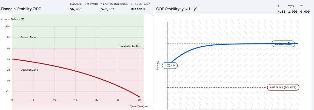
Widget realized by Google Gemini.

Example: Bank Account with Embezzlement

Let’s explore how to model and analyze the behavior of a bank account that is simultaneously accruing interest and experiencing consistent withdrawals due to embezzlement. This scenario helps illustrate how differential equations can be used to understand and predict real-world financial situations.

Let’s consider the following scenario where:

• y(t) is the amount of money in a bank account at time t (usually measured in years).
• r is the continuous annual interest rate on the account.
• w is the constant rate at which money is being embezzled from the account (the amount of money being stolen per unit time, e.g., dollars per day, euros per hour, etc.).

  Suppose a bank teller is illicitly withdrawing funds from a customer’s bank account without their knowledge or voluntary consent. The customer continues to accrue interest on their account balance at a continuous rate r, but the ongoing embezzlement at rate w affects the overall growth of the account. We aim to model the evolution of the account balance over time and understand under what conditions the balance will ultimately increase or decrease.

Mathematical Modeling

The rate of change of the account balance y(t) over time can be expressed as the difference between the interest earned and the amount being embezzled: $\frac{dy}{dt} = ry -w$ where:

• ry: Represents the rate at which the account balance increases due to continuous interest. The growth is proportional to the current balance y(t).
• −w: Represents the constant rate at which money is being embezzled from the account, steadily reducing the balance.

Analysis of the ODE

1. Autonomous Nature: This equation is a first-order linear autonomous ODE because it relates the derivative $\frac{dy}{dt}$ to the function y(t) itself and does not explicitly depend on the independent variable t (the rules of the account don’t change depending on what year it is).

   An autonomous ODE is one where the rate of change of the dependent variable depends solely on the dependent variable itself and not explicitly on the independent variable.

2. Finding Critical Points (Equilibrium Solutions): Critical points occur when the rate of change of the dependent variable is exactly zero (the account is stagnant): $\frac{dy}{dt} = 0 ⇒ ry -w = 0 ↭[\text{Solving for y:}] y = \frac{w}{r}$ (Refer to Figure 2 for a visual representation and aid in understanding it). Hence, $y = \frac{w}{r}$ is the equilibrium solution or critical point.

   At this precise balance, the amount of interest earned exactly offsets the amount being embezzled, resulting in a net zero change in the account balance over time.

   

   Arrows indicating the direction of y(t). Upwards for y > w/r, and downwards for y < w/r

3. Behaviour of the solution. To understand how the account balance changes over time, we analyze the sign of $\frac{dy}{dt}$ for values of y above and below the critical point threshold.

• When $y > \frac{w}{r}$, the function ry -w is positive, meaning $\frac{dy}{dt} > 0$. The solution is increasing, which means the bank account balance grows over time.

  If the bank account has more than w/r (the critical point threshold), the account balance increases over time because the interest earned per unit time exceeds the embezzlement rate. The lazy customer may never notice the embezzlement immediately due to the increasing balance.

• If $y < \frac{w}{r}$, the function ry -w is negative, meaning $\frac{dy}{dt} < 0$. The solution is decreasing, meaning that the bank account balance is shrinking over time.

  If the bank account has less than w/r (the critical point), the account balance diminishes because the constant losses due to embezzlement outweigh the interest gains. The account will eventually deplete, potentially leading to severe financial issues.

Solving the Differential Equation Explicitly

To find the exact formula for the account balance at any given time, we can solve the ODE using the separation of variables technique.

1. Separate Variables: $\frac{dy}{dt} = ry-w ↭ \frac{dy}{ry-w} = dt$
2. Integrate Both Sides: $\int \frac{dy}{ry-w} = \int dt ↭[Use u-substitution on the left side, u = ry -w⇒ du = rdy] \frac{1}{r}\int \frac{du}{u} = t + C ↭ \frac{1}{r}ln|u| = t + C ↭ \frac{1}{r}ln|ry-w| = t + C$
3. Solve for y. Multiply both sides by r: ln|ry -w| = rt + rC.
   Exponentiate both sides to eliminate the natural logarithm: $|ry -w| = e^{rt}e^{rC} \iff ry -w = ±e^{rC}e^{rt}$.
   Drop the absolute value by absorbing the ± into the constant. Let $A = \pm e^{rC}$, $ry = w + Ae^{rt}$.
   $y = \frac{w}{r} + \frac{A}{r}e^{rt}$.
   Since $ \frac{A}{r}e^{rt}$ is just another constant, let’s rename it C: $y = \frac{w}{r} + Ce^{rt}$
4. Apply initial conditions.
   Let’s the starting balance at time t = 0 be y(0) = y₀, $y_0 = \frac{w}{r}+ Ce^{r·0}↭ y_0 = \frac{w}{r}+ C ⇒ C = y_0 -\frac{w}{r}$
5. Final Explicit Solution. Substitute C back into our general equation, $\boxed{y(t) = \frac{w}{r}+(y_0-\frac{w}{r})e^{rt}}$

Final Interpretation of the Model:

The fate of the account relies entirely on the initial balance $y_0$ compared to the critical threshold $\frac{w}{r}$

1. The Hidden Crime. If the starting balance is large enough $y_0 > \frac{w}{r} ⇒ y_0-\frac{w}{r} > 0$. As $t \to \infty$, the term $e^{rt} \to \infty$ grows to infinity, pulling y(t) up with it. The account balance grows exponentially over time (without bound). The interest earned not only compensates for the embezzlement but also contributes to substantial growth of the account. The customer may not notice and be completely oblivious to the theft due to the increasing balance.
2. The Stagnant Account. If the balance perfectly matches the critical point, $y_0 = \frac{w}{r} \implies y(t) = \frac{w}{r}$. The account balance remains flat forever. The customer might just assume their interest rate is 0%, effectively masking the embezzlement.
3. The Doomed Account. If the starting balance is below the threshold $y_0 < \frac{w}{r} \implies y_0-\frac{w}{r} < 0$. As $t \to \infty$, the term $e^{rt} \to \infty$ drives the balance towards negative infinite. In practical terms, the account cannot have an infinite negative balance. Practically, account balance will decrease and eventually hit zero, leading to bounced checks, overdrafts, and the ultimate discovery of the crime!

Widget realized by Google Gemini.

Bibliography

1. NPTEL-NOC IITM, Introduction to Galois Theory.
2. Algebra, Second Edition, by Michael Artin.
3. LibreTexts, Calculus and Calculus 3e (Apex). Abstract and Geometric Algebra, Abstract Algebra: Theory and Applications (Judson).
4. Field and Galois Theory, by Patrick Morandi. Springer.
5. Michael Penn, and MathMajor.
6. Contemporary Abstract Algebra, Joseph, A. Gallian.
7. YouTube’s Andrew Misseldine: Calculus. College Algebra and Abstract Algebra.
8. MIT OpenCourseWare [18.03 Differential Equations, Spring 2006], YouTube by MIT OpenCourseWare.
9. Calculus Early Transcendentals: Differential & Multi-Variable Calculus for Social Sciences.