Existence and Uniqueness Theorem

Any fool can criticize, complain, and condemn— and most fools do. But it takes character and self-control to be understanding and forgiving, Dale Carnegie

Recall. Algebraic and differential equations.

An algebraic equation is a mathematical statement asserting that two algebraic expressions are equal.. These expressions are constructed using:

1. Dependent and independent variables. Variables are symbols representing unknown quantities. Variables can be:
   Independent Variables: Variables or input that can be chosen (or change) freely.
   Dependent Variables: Variables that depend on the independent variables.
2. Constants. Fixed numerical values that do not change, e.g., 2, π, 7.
3. Algebraic operations. Operations such as addition, subtraction, multiplication, division, exponentiation, powers, and root.

An algebraic equation typically has the following general form: Expression₁ = Expression₂, where the two expressions are set equal to each other.

Examples: y = 2x + 4 (simple linear equation, represents a straight line with a slope of 2 and a y-intercept of 4), ax² + bx + c = 0 (quadratic equation, it represents a parabola), $ln(xy + t) = z·sin(\sqrt{x})$.

Definition. A differential equation is an equation that involves one or more functions and their derivatives. It relates the function itself (the dependent variable), its derivatives with respect to one or more independent variables (rates of change), and the independent variable(s) themselves, e.g., $\frac{dy}{dx} = 3x +5y, y' + y = 4xcos(2x), \frac{dy}{dx} = x^2y+y, etc.$

If an algebraic equation is a “snapshot” of a relationship, a differential equation is the “instruction manual” for how that relationship moves and changes.

Key Components (e.g., $\frac{dy}{dx} = 3x +5y$):

• Dependent variables: The function y (or y(x)) we are trying to find or solve for. Variable(s) (y) that depend on one or more other variables.
• Independent variables: Variable(s) (x) upon which the dependent variables depend and we differentiate with respect to (often time or space).
• Derivatives: Expressions like $\frac{dy}{dx}$ or y’ that represent the rate at which the dependent variable (y) change with respect to the independent variable (x).

Existence and Uniqueness Theorem

The Existence and Uniqueness Theorem (often called the Picard–Lindelöf Theorem) provides crucial insight into the behavior of solutions to first-order differential equations ODEs. It is the “safety net” of differential equations. It tells us precisely when we can trust that an initial value problem (IVP) has exactly one solution.

The Theorem Statement

For a first-order ODE $y' = f(x, y)$ with an initial condition $y(x_0) = y_0$:

1. Existence: If $f(x, y)$ is continuous in some rectangular region containing the point $(x_0, y_0)$, then a solution exists.
2. Uniqueness: If the partial derivative $\frac{\partial f}{\partial y}$ is also continuous in that same region, then the solution is unique.

The Geometric Consequence: If these conditions are met, integral curves cannot cross or touch one another. If two curves were to intersect at a point $(x, y)$, they would both satisfy the same initial condition at that point, which would violate the “uniqueness” part of the theorem.

Case Study 1: The “Well-Behaved” Equation

ODE: $y' = 1 + x - y$

1. Analysis via Theorem

• $f(x, y) = 1 + x - y$: This is a polynomial function, which is continuous everywhere in the $\mathbb{R}^2$ plane.
• $\frac{\partial f}{\partial y} = -1$: This is a constant function, which is also continuous everywhere.

Thus, the Existence and Uniqueness Theorem guarantees that for any point $(x_0, y_0)$ you pick (i.e., any intial condition $y(x_0) = y_0$), there is exactly one solution curve passing through it. The “flow” of the direction field will never tangle or overlap. In other words, two solution (integral) curves cannot cross or touch each other, as this would violate uniqueness.

2. Analytical Solution: Integrating Factors

Let’s now find an explicit solution to the ODE by using the method of integrating factors.

The differential equation is: y’ = 1 + x -y ↭[Bring all terms involving y to one side] y’ + y = 1 + x. This is a linear ODE of the form (basically, we have rewritten it in standard form): y’ +p(x)y = q(x) where p(x)= 1 and q(x) = 1 + x.

Step 1: Find the Integrating Factor $\mu(x)$: $μ(x) = e^{\int p(x)dx} = e^{\int 1dx}= e^x$.

Step 2: Multiply both sides of the equation by the Integrating Factor: $e^x·y' + e^x·y = (1+x)e^x$.
Recognize the left-hand as a product derivative of e^x·y: $\frac{d}{dx}(e^x·y) = (1+x)e^x$

Step 3: Integrate both sides with respect to x: $e^x·y = \int (1+x)e^xdx = \int e^xdx + \int xe^xdx$
The first integral is straightforward: $\int e^xdx = e^x$.
The second integral requires integration by parts. Let u = x and dv = e^xdx, so that du = dx and v = e^x.
$\int xe^xdx = xe^x -\int e^xdx = xe^x -e^x$.
Combine results and the full integral becomes: $\int (1+x)e^xdx = e^x + (xe^x -e^x) = xe^x + C$.
Substitute this back into the equation: $(\star)~ e^x·y = xe^x + C$ where C is the constant of integration.

Step 4: Solve for $y$. Finally, divide both sides by $e^x$ (which is always positive) to solve for y: $e^x y = xe^x + C \implies \boxed{y = x + Ce^{-x}}$

3. Geometric Interpretation (Asymptotic Behavior)

As $x \to \infty$, the term $Ce^{-x}$ decays to zero. Therefore, the solution asymptotically approaches the line y = x as $x \to \infty$. This means that every single solution, regardless of its starting constant $C$, eventually merges toward the line $y = x$. This confirms our earlier observation of the “attractor” in the direction field.

Case Study 2: The Failure of Uniqueness

If an initial solution is given, such as y(x₀) = y₀, we can substitute these values into the general solution to find the specific value of C. For instance, if y(0) = y₀, we have y₀ = 0 + Ce⁰ = C, so C = y₀. Therefore, the solution simplifies to y = x + y₀e^-x.

More specifically, if y₀ = 0, then the constant C equals 0, and the solution simplifies to y = x with slope 1 (y’ = 1), which is also the solution we obtained geometrically.

Solve the Differential Equation xy’ = y -1

Let’s solve the first-order ordinary differential equation (ODE): $xy' = y - 1$.

1. Analytical Solution: Separation of Variables

First, we solve the equation to see what the curves look like.

The differential equation can be rewritten as $x·\frac{dy}{dx} = y - 1 \implies \frac{dy}{dx} =\frac{y-1}{x}$

This is a separable differential equation, meaning we can separate the variables y and x to solve it.

Let’s proceed by separating the terms involving y on one side and those involving x on the other side: $\frac{dy}{y-1} = \frac{dx}{x}$

Next, we integrate both sides: $\int \frac{dy}{y-1} = \int \frac{dx}{x} ↭[\text{This yields}] ln|y-1| = ln|x| + C$ where C is the constant of integration.

Next, we exponentiate both sides to eliminate the logarithms: $e^{ln|y-1|} = e^{ln|x|+ C} \implies |y-1| = e^C|x|$. Since e^C is always a positive constant, we can replace it with a new constant C (abusing mathematical notation).

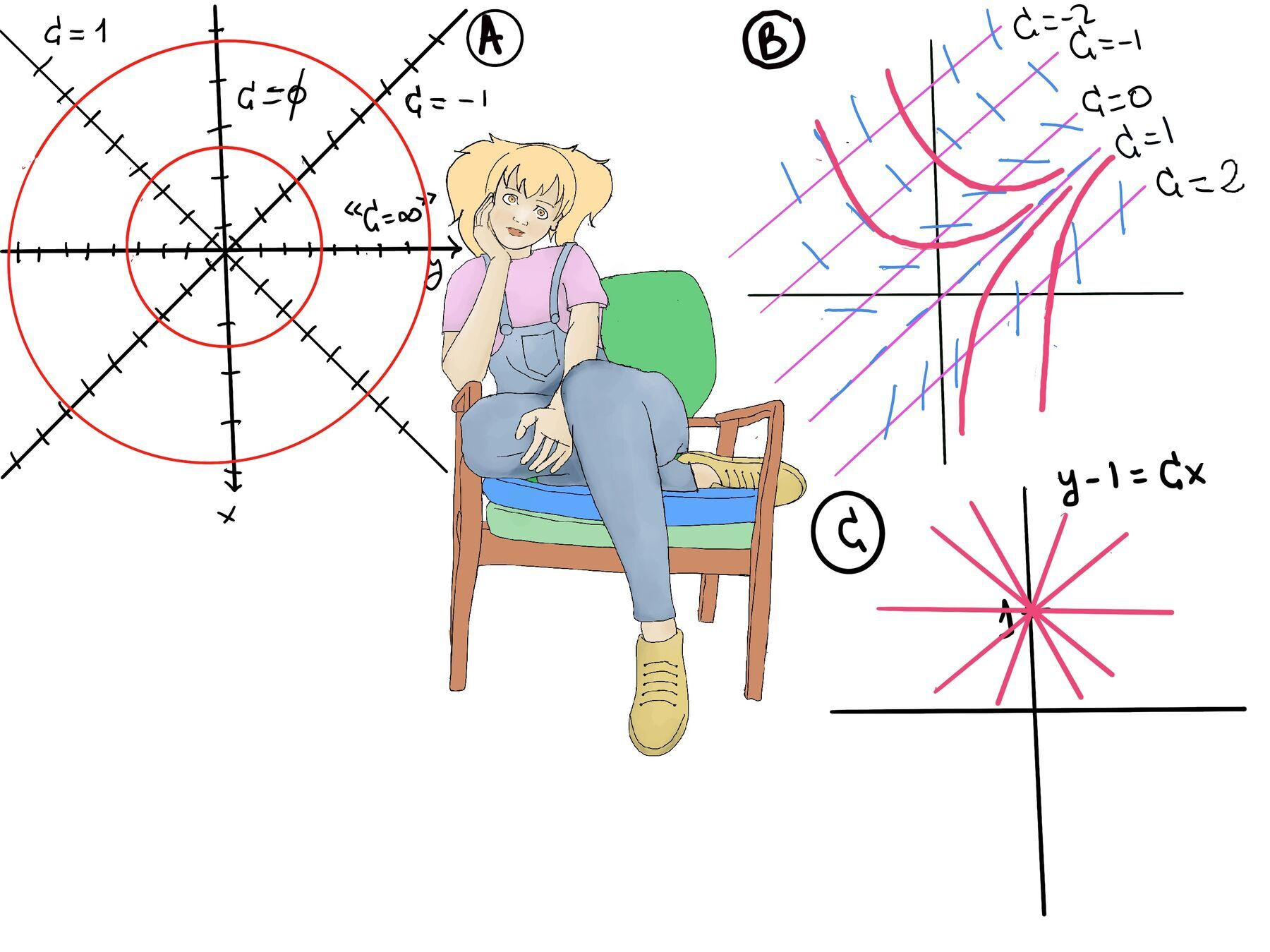
At this point, we drop the absolute values, leading to y - 1 = Cx where C is a constant which might absorb the sign difference (both/one of x and/or y-1 are positive or negative y -1 = Cx and/or y -1 = -Cx) and is determined by initial conditions (Refer to Figure C for a visual representation and aid in understanding it).

Thus, the general solution to the differential equation is y(x) = 1 + Cx.This represents a family of straight lines with varying slopes determined by the constant C. Each line passes through the point (0, 1) when x = 0, and the slope of each line is given by C.

2. Analysis via the Existence and Uniqueness Theorem

The existence and uniqueness theorem for differential equations states that, under certain conditions, a unique solution exists for an initial value problem (an ordinary differential equation together with an initial condition). Specifically, for a first-order equation of the form: $y' = f(x, y)$ with an initial condition $y(x_0) = y_0$:

1. Existence: If $f(x, y)$ is continuous in some rectangular region containing the point $(x_0, y_0)$, then a solution exists.
2. Uniqueness: If the partial derivative $\frac{\partial f}{\partial y}$ is also continuous in that same region, then the solution is unique.

For our equation in its rewritten form: $\frac{dy}{dx} = \frac{y-1}{x}$ or $y' = \frac{y-1}{x}$. We observe that the right-hand side of this equation, $\frac{y-1}{x}$, is not defined when x = 0. This introduces a singularity at x = 0 where the function is obviously not continuous. Therefore,

• At any point where $x \neq 0$: $f(x, y)$ and $\frac{\partial f}{\partial y} = \frac{1}{x}$ are continuous. The theorem holds; it guarantees a unique solution passing through any point $(x_0, y_0)$ where $x_0 \ne 0$/
• At $x = 0$: The function $f(x, y)$ is undefined (division by zero). The theorem fails.

3. Interpreting the Singularity

What happens at the vertical line $x = 0$ (the $y$-axis)?

1. At the point $(0, 1)$: If we plug $x=0$ and $y=1$ into the original ODE ($xy' = y-1$), we get $0 \cdot y' = 1-1$, or $0 = 0$. This equation is true for any value of $y'$. This is why infinitely many lines ($y = Kx + 1$) can pass through this single point. Uniqueness fails.

   Specifically, for x = 0, any value of C would satisfy the equation y = 1 + Cx, because the equation degenerates to y = 1 when x = 0. Therefore, we have infinitely many solutions passing through (0, 1), meaning that uniqueness fails at this point.

2. At any other point on the y-axis (e.g., $(0, 2)$): Plugging in $x = 0$ and $y = 2$ gives $0 = 2 - 1$, or $0 = 1$. This is impossible. Therefore, no solution exists that passes through $(0, 2)$.

Final Insight

There are three possibilities for an initial value problem:

1. ✅ One unique solution (ideal case).
2. ❌ No solution.
3. ❌ Infinitely many solutions.

The Existence and Uniqueness Theorem tells us when we are guaranteed to be in Case 1.

Bibliography

1. NPTEL-NOC IITM, Introduction to Galois Theory.
2. Algebra, Second Edition, by Michael Artin.
3. LibreTexts, Calculus and Calculus 3e (Apex). Abstract and Geometric Algebra, Abstract Algebra: Theory and Applications (Judson).
4. Field and Galois Theory, by Patrick Morandi. Springer.
5. Michael Penn, and MathMajor.
6. Contemporary Abstract Algebra, Joseph, A. Gallian.
7. YouTube’s Andrew Misseldine: Calculus. College Algebra and Abstract Algebra.
8. MIT OpenCourseWare [18.03 Differential Equations, Spring 2006], YouTube by MIT OpenCourseWare.
9. Calculus Early Transcendentals: Differential & Multi-Variable Calculus for Social Sciences.