Euler's Method. Numerical Approximation for ODEs

Pure mathematics is, in its way, the poetry of logical ideas. Do not worry about your difficulties in mathematics, I assure you that mine are still greater, Albert Einstein

Recall. Algebraic and differential equations.

An algebraic equation is a mathematical statement asserting that two algebraic expressions are equal.. These expressions are constructed using:

1. Dependent and independent variables. Variables are symbols representing unknown quantities. Variables can be:
   Independent Variables: Variables or input that can be chosen (or change) freely.
   Dependent Variables: Variables that depend on the independent variables.
2. Constants. Fixed numerical values that do not change, e.g., 2, π, 7.
3. Algebraic operations. Operations such as addition, subtraction, multiplication, division, exponentiation, powers, and root.

An algebraic equation typically has the following general form: Expression₁ = Expression₂, where the two expressions are set equal to each other.

Examples: y = 2x + 4 (simple linear equation, represents a straight line with a slope of 2 and a y-intercept of 4), ax² + bx + c = 0 (quadratic equation, it represents a parabola), $ln(xy + t) = z·sin(\sqrt{x})$.

Definition. A differential equation is an equation that involves one or more functions and their derivatives. It relates the function itself (the dependent variable), its derivatives with respect to one or more independent variables (rates of change), and the independent variable(s) themselves, e.g., $\frac{dy}{dx} = 3x +5y, y' + y = 4xcos(2x), \frac{dy}{dx} = x^2y+y, etc.$

If an algebraic equation is a “snapshot” of a relationship, a differential equation is the “instruction manual” for how that relationship moves and changes.

Key Components (e.g., $\frac{dy}{dx} = 3x +5y$):

• Dependent variables: The function y (or y(x)) we are trying to find or solve for. Variable(s) (y) that depend on one or more other variables.
• Independent variables: Variable(s) (x) upon which the dependent variables depend and we differentiate with respect to (often time or space).
• Derivatives: Expressions like $\frac{dy}{dx}$ or y’ that represent the rate at which the dependent variable (y) change with respect to the independent variable (x).

Solving differential equations

To solve ordinary differential equations (ODEs), several methods can be employed, each suited to different types of equations. Here are some of the key methods:

• Separation of Variables. This method is used for ODEs where the algebraic expression can be factored into a function of $x$ times a function of $y$, $\frac{dy}{dx} = g(x)h(y)$. By separating the variables to opposite sides of the equation, you can integrate both sides separately: $\int \frac{dy}{h(y)} = \int g(x)dx + C$

• Integrating Factors. This powerful technique applies strictly to linear first-order ODEs, $\frac{dy}{dx} + P(x)y = Q(x)$. The idea is to multiply the entire equation by an integrating factor μ(x) = $e^{\int P(x)dx}$, which simplifies the left-hand side into a product derivative, making the equation easier to solve: $\frac{d}{dx}(y·μ(x)) = Q(x)·μ(x)$. Integrating both sides with respect to x yields the solution.

• Exact Differential Equations. These are ODEs that can be expressed in the form of a total differential of a multivariable potential function, M(x, y)dx + N(x, y)dy = 0, where the exactness condition $\boxed{\frac{∂M}{∂y} = \frac{∂N}{∂x}}$ must be satisfied. If exact, you integrate $M$ with respect to $x$ (and $N$ with respect to $y$) to reverse-engineer the original potential function $f(x, y)$. The implicit solution is defined as $f(x,y) = C$.

• Substitution Methods (e.g., Bernoulli Equations). Sometimes an ODE doesn’t fit the above categories but can be transformed into one that does via substitution. For example, a Bernoulli equation takes the form $y' + P(x)y = Q(x)y^n$. By using the substitution $v = y^{1-n}$, the equation is transformed into a standard linear ODE, which can then be solved using an Integrating Factor.

• Geometric Interpretations. This approach involves visualizing the solution in the phase plane or using graphical methods to understand the behavior of the solutions. For example, in autonomous differential equations, the phase plane can help in understanding the equilibrium points and the stability of the solutions.

• Numerical Methods. For ODEs that cannot be solved analytically, numerical methods are used to find approximate solutions.

Euler’s Method: Numerical Approximation for ODEs

Euler’s method is the most fundamental numerical technique for approximating the solution to a first-order Initial Value Problem (IVP): $y' = f(x, y), \quad y(x_0) = y_0$.

Unlike analytical methods that seek an explicit formula for y(x), Euler’s method generates an approximation by creating a sequence of discrete points (x_k, y_k) that estimate the true solution at discrete points. More precisely, each y_k estimates the value of the true solution y(x_k).

Euler's method approximates the continuous solution curve by linking together a series of short tangent lines (Refer to Figure 1 for a visual representation and aid in understanding it). Each new point is determined by calculating the slope of the tangent line at the previous point.

The slope at any point $(x_k, y_k)$ is determined exactly by the given differential equation y′ = f(x, y). The method progresses from one point to the next by taking small, uniform steps of size h along the x-axis.

Method Outline

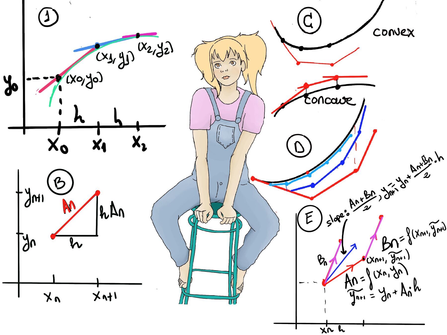
Given the differential equation of the form: y’ = f(x, y) and an initial condition y(x₀) = y₀, Euler’s method approximates y at points x₁, x₂, ···, x_N. The basic idea is to use the slope at $(x_n, y_n)$ to estimate y at the next point $x_{n+1}$ of the sequence using the following steps:

1. Start with the initial point. Begin with $(x_0, y_0)$ where $y_0$ is the known initial value of the solution at $x_0$.
2. Choose a Step Size h: The value of h determines the horizontal interval between successive points. A smaller h generally leads to better accuracy but obviously requires more computations effort (which is less of a concern for modern computers, they have evolved tremendously over the years, becoming incredibly powerful).
3. Compute the Slope: At each step n, compute the slope A_n of the tangent line at (x_n, y_n) by plugging the coordinates into the differential equation: A_n = f(x_n, y_n).
4. Update the Values: The next y-value, y_n+1 is calculated using the slope at (x_n, y_n) and the step size: y_n+1-y_n = hA_n or equivalently y_n+1 = y_n + hA_n. Similarly, the next x-value is: $x_{n+1}=x_n + h$.
5. Repeat the Process: Continue/Iterate this process to compute the sequence of points (x₁, y₁), (x₂, y₂), ··· (x_n, y_n), ···, generating a numerical approximation of the solution curve (Refer to Figure B for a visual representation and aid in understanding it).

To summarize, the iterative formulas are: $\boxed{x_{n+1} = x_n + h \quad \text{and} \quad y_{n+1} = y_n + h \cdot f(x_n, y_n)}$

Solved examples

• Consider the differential equation $y' = x^2 - y^2$. Given the initial condition $y(0) = 1$ and a step size of $h = 0.1$, we will approximate $y$ at $x = 0.3$ and $x = 0.4$.

Step-by-step table of calculations:

Using the table, the approximated value at $x = 0.3$ is $y_3 \approx y_2 + hA_2 \approx 0.82 −0.06324 = 0.75676$. To find the approximated value at $x = 0.4$, we perform one more iteration: $y_4 = y_3 + hA_3 = 0.75676 - 0.048268 = \mathbf{0.70849}$

Discussion of the Results

Euler’s method provides a straightforward approach to approximating solutions of first-order ODEs. While simple and easy to implement, its accuracy depends heavily on the step size h and the geometric behavior of the true solution.

• Convex Solutions ($y'' > 0$): If the true solution is curving upward, the tangent lines will sit below the curve. Therefore, Euler’s approximation tends to underestimate the true value.

• Concave Solutions ($y'' < 0$): If the true solution is curving downward, the tangent lines will sit above the curve. Therefore, Euler’s approximation tends to overestimate the true value (Refer to Figure C for a visual representation and aid in understanding it).

Applying this to our example:

In our example, to determine the convexity, we calculate the second derivative using implicit differentiation and the Chain Rule: $y'' = \frac{d}{dx}(y') = \frac{d}{dx}(x^2-y^2) = 2x -2yy'.$

Evaluate this at our initial condition (x₀ = 0, y₀ = 1): y(0) = 1 (Initial condition), y’(0) = A₀ = -1, y’’(0) =[y’’ = 2x -2yy’] 2·0 -2·1·(-1) = 2. Since y′′(0) = 2 > 0, the exact solution is convex near x = 0. We can confidently conclude that Euler’s method will underestimate the true solution in the initial steps.

Error Analysis

Euler’s method approximates the solution curve by constructing a series of tangent line segments, moving from one point to the next based on the local slope of the solution at the current point.

Each tangent line is a linear approximation, and as such, the error introduced at each step depends on how much the true solution deviates from linearity over that interval. Therefore, its accuracy can vary depending on the step size and the nature of the solution curve. For smoother (slowly changing) functions, Euler’s method performs better, while for more complex functions, smaller steps (halve the step side, halve the error, refer to Figure D) or more advanced numerical methods (like Runge-Kutta) may be needed for improved accuracy and stability.

• Approximating $y' = x + 2y$ using Euler’s Method

Let’s consider the differential equation $y' = x + 2y$, with the initial condition $y(0) = 0$. We want to approximate $y(0.4)$ using a step size of $h = 0.1$.

Euler’s method is a fundamental numerical technique used to approximate solutions to ordinary differential equations (ODEs) when an analytical solution is difficult, costly or impossible to obtain.

Step-by-step table of calculations $\boxed{x_{n+1} = x_n + h \quad \text{and} \quad y_{n+1} = y_n + h \cdot f(x_n, y_n)}$:

After four steps, the approximated value at x = 0.4 is y₄ ≈ 0.032 + 0.0364 = 0.0684.

Verification with the Exact Solution

To evaluate the accuracy of our numerical approximation, let’s solve the differential equation analytically.

1. Rewrite the equation in standard linear form: y’ -2y = x.
2. Compute the integrating factor μ(x) = $e^{\int -2dx} = e^{-2x}$
3. Multiply both sides by μ(x): $e^{-2x}y'-2e^{-2x}y = e^{-2x}x↭ \frac{d}{dx}(e^{-2x}y)= e^{-2x}x$
4. Integrate Both Sides: $e^{-2x}y = \int e^{-2x}xdx = $[Integration by parts. u = x ⇒ du = dx, $dv = e^{-2x}dx, v = \frac{-1}{2}e^{-2x}$] = $\frac{-1}{2}xe^{-2x} -\int \frac{-1}{2}e^{-2x}dx = \frac{-1}{2}xe^{-2x} +\int \frac{1}{2}e^{-2x}dx = \frac{-1}{2}xe^{-2x} - \frac{1}{4}e^{-2x} + C$. In conclusion, $e^{-2x}y = \frac{-1}{2}xe^{-2x} -\frac{1}{4}e^{-2x} + C$
5. Solve for y: $y = \frac{-1}{2}x - \frac{1}{4} + Ce^{2x}$
6. Apply Initial Conditions y(0) = 0, $0 = \frac{-1}{2}0 -\frac{1}{4} + Ce^{2·0}⇒ 0 = -\frac{1}{4} + C⇒\text{Solve for C: } C = \frac{1}{4}.$ Final Solution = $\boxed{y = \frac{1}{4}e^{2x} -\frac{1}{2}x -\frac{1}{4}}$
7. Compute y(0.4): $y(0.4) = \frac{1}{4}e^{2·0.4} - \frac{1}{2}0.4 - \frac{1}{4} = 0.25(2.22554) −0.2 −0.25 \approx 0.55639−0.45=0.106399.$

Conclusion: Our Euler's method approximation is y(0.4) ≈ 0.0684, whereas the exact value is approximately 0.106399. The discrepancy indicates that Euler's method with h = 0.1 is not very accurate for this problem over this interval.

Why does this happen? The exact solution involves an exponential term e^2x, with grows rapidly. Euler's method, relying on purely linear tangent approximations, with a relatively large step size h = 0.1, struggles to capture this rapid, compounding change. The error accumulates at each step, leading to significant deviation from the exact solution.

Geometric Proof of Underestimation (Convexity Check)

We can prove mathematically that Euler’s method will fall short. We calculate the second derivative:

$y'' = \frac{d}{dx}(y') = \frac{d}{dx}(x+2y) = 1 + 2y'$.

At our starting point $(0, 0)$, the slope is $y' = 0 + 2\cdot 0 = 0$, hence $y''(0) = 1 + 2(0) = 1$

Since $y'' > 0$, the solution curve is convex (curving upward) near $x = 0$. Tangent lines drawn on a convex curve always sit below the curve, proving that Euler’s method will always underestimate the true solution here.

Improving the Approximation

1. Smaller Step Size. Using a smaller step size h would improve the accuracy. It forces the tangent lines to recalculate more frequently, hugging the true curve tighter. For instance, halving the step to h = 0.05 will roughly halve the global error, though it doubles the computational effort.
2. Higher-Order Methods: Employing methods like the Improved Euler’s Method (also known as Heun’s Method) or the Runge-Kutta methods would yield vastly better approximations. These methods account for the curvature of the solution between steps, drastically reducing the error without needing microscopically small step sizes.

Bibliography

1. NPTEL-NOC IITM, Introduction to Galois Theory.
2. Algebra, Second Edition, by Michael Artin.
3. LibreTexts, Calculus and Calculus 3e (Apex). Abstract and Geometric Algebra, Abstract Algebra: Theory and Applications (Judson).
4. Field and Galois Theory, by Patrick Morandi. Springer.
5. Michael Penn, and MathMajor.
6. Contemporary Abstract Algebra, Joseph, A. Gallian.
7. YouTube’s Andrew Misseldine: Calculus. College Algebra and Abstract Algebra.
8. MIT OpenCourseWare [18.03 Differential Equations, Spring 2006], YouTube by MIT OpenCourseWare.
9. Calculus Early Transcendentals: Differential & Multi-Variable Calculus for Social Sciences.