It ain’t about how hard you can hit. Its about how hard you can get hit, and how much you can take, and keep moving forward, Rocky Balboa

You can only grow if you’re willing to feel awkward and uncomfortable when you try something new, Brian Tracy

Recall. Algebraic and differential equations.

An algebraic equation is a mathematical statement asserting that two algebraic expressions are equal.. These expressions are constructed using:

Dependent and independent variables. Variables are symbols representing unknown quantities. Variables can be:
Independent Variables: Variables or input that can be chosen (or change) freely.
Dependent Variables: Variables that depend on the independent variables.
Constants. Fixed numerical values that do not change, e.g., 2, π, 7.
Algebraic operations. Operations such as addition, subtraction, multiplication, division, exponentiation, powers, and root.

An algebraic equation typically has the following general form: Expression₁ = Expression₂, where the two expressions are set equal to each other.

Examples: y = 2x + 4 (simple linear equation, represents a straight line with a slope of 2 and a y-intercept of 4), ax² + bx + c = 0 (quadratic equation, it represents a parabola), $ln(xy + t) = z·sin(\sqrt{x})$.

Definition. A differential equation is an equation that involves one or more functions and their derivatives. It relates the function itself (the dependent variable), its derivatives with respect to one or more independent variables (rates of change), and the independent variable(s) themselves, e.g., $\frac{dy}{dx} = 3x +5y, y' + y = 4xcos(2x), \frac{dy}{dx} = x^2y+y, etc.$

If an algebraic equation is a “snapshot” of a relationship, a differential equation is the “instruction manual” for how that relationship moves and changes.

Key Components (e.g., $\frac{dy}{dx} = 3x +5y$):

Dependent variables: The function y (or y(x)) we are trying to find or solve for. Variable(s) (y) that depend on one or more other variables.
Independent variables: Variable(s) (x) upon which the dependent variables depend and we differentiate with respect to (often time or space).
Derivatives: Expressions like $\frac{dy}{dx}$ or y’ that represent the rate at which the dependent variable (y) change with respect to the independent variable (x).

Geometrical analysis

Solving differential equations

To solve ordinary differential equations (ODEs), several methods can be employed, each suited to different types of equations. Here are some of the key methods:

Separation of Variables. This method is used for ODEs where the algebraic expression can be factored into a function of $x$ times a function of $y$, $\frac{dy}{dx} = g(x)h(y)$. By separating the variables to opposite sides of the equation, you can integrate both sides separately: $\int \frac{dy}{h(y)} = \int g(x)dx + C$
Integrating Factors. This powerful technique applies strictly to linear first-order ODEs, $\frac{dy}{dx} + P(x)y = Q(x)$. The idea is to multiply the entire equation by an integrating factor μ(x) = $e^{\int P(x)dx}$, which simplifies the left-hand side into a product derivative, making the equation easier to solve: $\frac{d}{dx}(y·μ(x)) = Q(x)·μ(x)$. Integrating both sides with respect to x yields the solution.
Exact Differential Equations. These are ODEs that can be expressed in the form of a total differential of a multivariable potential function, M(x, y)dx + N(x, y)dy = 0, where the exactness condition $\boxed{\frac{∂M}{∂y} = \frac{∂N}{∂x}}$ must be satisfied. If exact, you integrate $M$ with respect to $x$ (and $N$ with respect to $y$) to reverse-engineer the original potential function $f(x, y)$. The implicit solution is defined as $f(x,y) = C$.
Substitution Methods (e.g., Bernoulli Equations). Sometimes an ODE doesn’t fit the above categories but can be transformed into one that does via substitution. For example, a Bernoulli equation takes the form $y' + P(x)y = Q(x)y^n$. By using the substitution $v = y^{1-n}$, the equation is transformed into a standard linear ODE, which can then be solved using an Integrating Factor.
Geometric Interpretations. This approach involves visualizing the solution in the phase plane or using graphical methods to understand the behavior of the solutions. For example, in autonomous differential equations, the phase plane can help in understanding the equilibrium points and the stability of the solutions.
Numerical Methods. For ODEs that cannot be solved analytically, numerical methods are used to find approximate solutions.

Geometrical View

Sketch and Solve $\frac{dy}{dx} = x + y$.

This equation is a classic example of how a direction field reveals a hidden “partition” in the behavior of solutions.

1. Qualitative Analysis (The Direction Field)

Let’s analyze and solve this first-order ordinary differential equation (ODE). We will start with a qualitative approach by sketching the direction field to understand the global behavior, and then proceed to solve the equation analytically.

What is a direction field? A direction field (or slope field) is a graphical tool that shows the slope of the solution curve $\frac{dy}{dx}$, at various points (x, y). This helps us visualize how solution curves “flow” (or “behave”) across the plane without explicitly solving the equation.

An isocline is a curve along which the slope $\frac{dy}{dx}$ remains constant. For our differential equation, we set the slope equal to a constant C, and we get $\frac{dy}{dx} = x + y = C$, each value of C corresponds to a different isocline.

Solving for y, we get y = -x + C. Thus, each isocline is a straight line of the form y = -x + C with a slope of −1. Each line corresponds to a different value of C and represents a set of points where the direction field has that exact slope.

Examples of Specific Isoclines: Let’s consider specific values of C to understand how the direction field behaves along different isoclines.

For C = 0, we have the equation of the isocline y = -x, meaning that along this line, the direction field has a constant slope of y’ = 0, i.e., the line segments in the direction field (solution curves near this line) are perfectly horizontal.
For C = -1, the isocline is y = -x - 1, meaning that on this line the direction field has a constant slope -1, indicating line segments inclined or angled downward (slanting) at a 45-degree angle, parallel to the isocline itself.
For C = 1, the isocline is y = -x + 1. The slope of the direction field along this line is one, so the line segments are inclined upward at 45-degrees.
For C = 2, the isocline is y = -x +2, the slope y’ = 2, indicating steeper upward line segments.
For C = -2, we get the line y = -x -2, meaning that on this line the direction field has a constant slope -2, representing steeper downward line segments (slopes) and so on.

Observing the “Partition” Effect

By analyzing these isoclines, we can deduce the behavior of the solution curves:

The Separatrix (y = −x − 1). Notice that when C = −1, the isocline is y = −x −1 and the slope is −1. Because the line’s slope matches the direction field’s slope, y = −x −1 is actually an exact, straight-line solution to the ODE. It acts as a hard boundary or partition.

Take the ODE, $\frac{dy}{dx} = x + y$. Now test the candidate function: y(x) = −x −1, y’(x) = -1 and we plug it into the ODE: x + (-x + 1) = -1. Therefore, y = −x −1 is an exact solution of the ODE. Note: The direction field slope given by the ODE is also −1.
Above the Partition (y > −x −1): Here, the solution curves are eventually pushed upward. $x \to \infty$, the solutions curve are inclined upwards, more and more steeply, growing without bound.
Below the Partition (y < −x −1): Here, the slope becomes increasingly negative. As $x \to \infty$, the solution curves are incline downwards, they fall steeper and steeper, decreasing without bound.
Looking Backward ($x \to -\infty$): No matter where a solution starts, if we trace it backward to the left, all solution curves flatten out and asymptotically approach the partition line y = −x −1.

2. Solving the Differential Equation Analytically

To deepen our understanding and rigorously verify our geometric observations, let’s solve the differential equation analytically: $\frac{dy}{dx} = x + y$.

We can rewrite the equation as: $\frac{dy}{dx}-y = x$. This is a linear first-order differential equation of the standard form: $\frac{dy}{dx} + P(x)y = Q(x)$ where P(x) = -1 and Q(x) = x.

Compute the integral factor: $μ(x) = e^{\int P(x)dx} = e^{\int -dx} = e^{-x}$
Multiply both sides of the ODE by the integrating factor μ(x): $e^{-x}\frac{dy}{dx}-e^{-x}y = e^{-x}x$
Recognize the Left Side as a the derivative of a product: $\frac{d}{dx}(e^{-x}y) = e^{-x}x$
Integrate both sides with respect to x: $e^{-x}y = \int e^{-x}xdx$
To evaluate the integral on the right, we use integration by parts (∫udv = uv −∫vdu): u = x ⇒ du = dx, $dv = e^{-x}dx \implies v = -e^{-x}.$
Applying this to our integral: $e^{-x}y = \int e^{-x}xdx = -xe^{-x}-\int -e^{-x}dx ⇒ e^{-x}y = -xe^{-x} - e^{-x} + C$
Sove explicitly for y. Multiply both sides by e^x: y = -x - 1 + Ce^x. The general solution to the differential equation is: y(x) = $-x - 1 + Ce^x$

Limit Analysis (Verifying the Asymptote)

Looking at the general solution, we can mathematically confirm our visual observations:

As $x \to -\infty$, the term $e^x \to 0$, Therefore, the term $Ce^x$ vanishes and y(x) ≈ -x - 1. This proves that all solution curves asymptotically approach the line y = −x −1 on the left side of the graph.
As $x \to \infty$, the term $e^x \to \infty$, so $Ce^x$ dominates the behaviour: If C > 0, the solution shoots up to +∞.
If C < 0, the solution dives down to −∞.
If C = 0, the exponential term disappears completely, leaving only the exact straight-line solution y = −x −1.

Geometrical View EDOs

Sketch and Solve $y' = \frac{-y}{x^2+y^2}$

This is a nonlinear ordinary differential equation (ODE) due to the presence of y² in the denominator. Solving this equation explicitly for y(x) in terms of elementary functions is quite challenging. However, we can gain significant insights by analyzing the isoclines and the behavior of the solutions.

1. Analyzing the isoclines

An isocline is a curve along which the slope y’ of the solution curves is constant. That is, all solution curves intersecting an isocline have the same slope at the points of intersection.

To find the isoclines, we set the slope y′ equal to a constant m and analyze the resulting equation: $\frac{-y}{x^2+y^2} = m$

Let’s break this down into two cases:

Case 1. The slope is zero, m = 0, the equation becomes $0 = \frac{-y}{x^2+y^2}$, which implies y = 0. Therefore, the x-axis (y = 0) is an isocline where the slope y’ = 0, meaning the line segments in the direction field are perfectly horizontal along the x-axis.
Case 2. The slope is non-zero, m ≠ 0, $\frac{-y}{x^2+y^2} = m ↭[\text{Multiplying both sides by x² + y²}] -y = m(x^2+y^2) ↭\frac{-1}{m}y = x^2 + y^2 ↭ x^2 + y^2 + \frac{1}{m}y = 0$
To identify this geometric shape, we complete the square for the y terms: $x^2 + (y+\frac{1}{2m})^2 = \frac{1}{4m^2}$. For each constant slope m ≠ 0, the isoclines is a circle centered along the y-axis at (0, $\frac{-1}{2m}$) with a radius of r = $\frac{1}{2|m|}$. The sign of m determines the position of the center along the y-axis.

Examples of Specific Isoclines

Let’s consider specific values of m to illustrate the isoclines:

m = -1 ⇒ We have a circle centered at (0, $\frac{1}{2}$) and radius $\frac{1}{2}$. Everywhere on this circle, the line segments in the direction field are inclined downwards at a 45-degree angle (slope y’ = -1).
m = 1 ⇒ We have a circle centered at (0, $\frac{-1}{2}$) and radius $\frac{1}{2}$. Everywhere on this circle, the line segments are inclined upwards at a 45-degree angle (slope y’ = 1).
m = -2 ⇒ We get a smaller circle centered at (0, $\frac{1}{4}$) with radius $\frac{1}{4}$. The line segments here are inclined steeper downward (slope y ′= −2).
m = 2 ⇒ We get a smaller circle centered at (0, $\frac{-1}{4}$) and radius $\frac{1}{4}$. The line segments here are inclined steeper upward (slope y′ = 2).

Note: All of these isocline circles pass through the origin (0, 0). However, because the denominator of our ODE is $x^2+y^2$ , the differential equation is undefined at the origin. It is a singular point.

2. Behavior of Solutions

By looking at the direction field generated by these circular isoclines, we can determine how the solutions behave globally.

The Trivial Solution: y = 0 is a constant solution of our EDO. Because of the Existence and Uniqueness Theorem, solutions starting on one side of the x-axis are “trapped” and will remain on that side (they cannot cross y=0, nor can they pass through the singularity at the origin).
y(x) = 0, then y’(x) = 0, and plug into the differential equation $\frac{-y}{x^2+y^2}=\frac{0}{x^2+0}=0 \iff 0 = 0$. This is true, so y(x) = 0 is indeed a solution.
The Existence and Uniqueness Theorem states that if the function and its partial derivative $\frac{\partial f}{\partial y}$ are continuous near $(x_0, y_0)$, then there is a unique solution passing through that point, and no other solution curve can cross it.
Away from the origin, the function is perfectly smooth, so f(x, y) is continuous, and $\frac{\partial f}{\partial y}$ is also continuous. Thus, the EUT applies everywhere except at the origin.
Therefore, solutions starting on one side of the x-axis are trapped and will remain on that side (they cannot cross y = 0, nor can they pass through the singularity at the origin).
Suppose a solution crosses the x‑axis at some point $(x_0, 0)$. The value of the solution is $y(x_0) = 0$, the slope is $y'(x_0) = \frac{-0}{x_0^2 + 0} = 0$. But the trivial solution y = 0 also passes through $(x_0, 0)$, and there can only be one solution through $(x_0, 0)$, and we already have one, the trivial one.
Solutions Above the x-axis (y > 0). The numerator -y is negative, and the denominator x² + y² is always positive. Thus, y’ < 0 (the slopes are always negative, so the solution is decreasing). As x increase, x² dominates the fraction, causing the magnitude of y’ to shrink toward 0. Therefore, solutions approach y = 0 asymptotically from above but never reach it (Refer to Figure ii for a visual representation and aid in understanding it).
Solutions Below the x-axis (y < 0). The numerator -y is positive and the denominator is always positive. Thus, y’ > 0 (the slopes are always positive, so the solution is increasing). As x increase, x² dominates again, and the magnitude of y’ decreases or shrinks toward 0. Solutions approach y = 0 asymptotically from below but never reach it.
Summary, all non-zero solutions flatten out (approach the x-axis) as x→∞, but never touch it. Solutions flatten out as they extend along the x-axis, reflecting the diminishing influence of y in the denominator compared to the unbounded growth of x².

Geometrical View EDOs

Solve and sketch y’ = y -2x with initial condition (1, 0)

Solve the Differential Equation

This is a linear first-order differential equation. We can solve it using an integrating factor.

Rewrite the Equation in Standard Linear Form y’ + P(x)y = Q(x): y’ - y = -2x
Integrating Factor: μ(x) = $e^{\int -1dx}=e^{-x}$.
Multiply Both Sides by Integrating Factor: $e^{-x}y' -e^{-x}y = -2xe^{-x} ↭ \frac{d}{dx}(e^{-x}·y) = -2xe^{-x}$
Integrate Both Sides: $\int \frac{d}{dx}(e^{-x}·y)dx = \int -2xe^{-x}dx ↭ e^{-x}·y = \int -2xe^{-x}dx ↭ e^{-x}·y = (2xe^{-x} + 2e^{-x}) + C$.
For the right side, use integration by parts: Let $u = -2x \Rightarrow du = -2dx; dv = e^{-x}dx \Rightarrow v = -e^{-x}$.
Then, $\int -2x e^{-x}dx = u v - \int vdu = (-2x)(-e^{-x}) - \int (-e^{-x})(-2)dx = 2x e^{-x} - 2\int e^{-x}dx = 2x e^{-x} + 2 e^{-x} + C$
So $e^{-x}y = 2x e^{-x} + 2 e^{-x} + C.$
Solve for y(x): Multiply by $e^{x}: y = 2x + 2 + C e^{x}$.
Apply Initial Condition y(1) = 0: $0 = 2·1 + 2 + C·e^{1} ⇒ C = -4e^{-1}$
Particular Solution Passing Through (1, 0): $\boxed{y(x) = 2x + 2 + -4e^{x-1}}$

2. Structure of the direction field

A direction field provides a visual representation of the slopes of the solution curves at various points in the plane. At each point (x, y), the slope is given directly by the ODE y’ = y - 2x.

An isocline is a curve where the slope is constant, say k: $y - 2x = k \quad\Longrightarrow\quad y = 2x + k.$

All isoclines are straight, parallel lines of slope 2.
Everywhere, along each line (y = 2x + k), the direction field has constant slope (y’ = y - 2x = k).

A special one is:

Zero-slope isocline: $y - 2x = 0 \Rightarrow y = 2x$. Along this line, (y’ = 0). This means whenever a solution curve crosses the line y = 2x, it must have a perfectly horizontal tangent (a local minimum or maximum).
The Exact Solution Isocline (k = 2): y= 2x + 2.
Notice what happens when we set k = 2. The line is y = 2x + 2 (which has a physical slope of 2). The direction field on this line also has a slope of k = 2.
Because the slope of the line matches the slope of the field, y = 2x + 2 is an exact, straight-line solution to the ODE!

Sample Slopes Table:

(x, y)	Slope	Slope
(0, 0), (0, 1), (0, 2), (0, 3)	0-0, 1-0, 2-0, 3-0	0, 1, 2, 3
(0, 0), (0, -1), (0, -2), (0, -3)	0-0, -1-0, -2-0, -3-0	0, -1, -2, -3
(1, 0), (1, 1), (1, 2), (1, 3)	0-2, 1-2, 2-2, 3-2	-2, -1, 0, 1
(1, 0), (1, -1), (1, -2), (1, -3)	0-2, -1-2, -2-2, -3-2	-2, -3, -4, -5

Geometric Interpretation of ODEs

3. Behavior of the Particular Solution

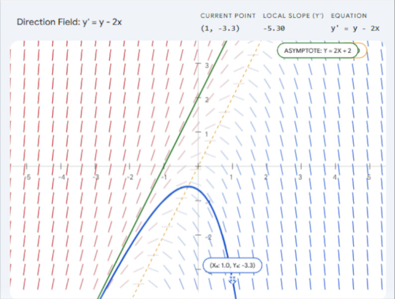
Let’s look at how our specific solution, $y(x) = 2x + 2 - 4e^{x-1}$, behaves geometrically starting from $(1, 0)$:

Moving Forward ($x \to \infty$): The exponential term $-4e^{x-1}$ dominates. Because it is negative, it pulls $y(x)$ downward rapidly. The curve dives off toward $-\infty$.
Moving Backward ($x \to -\infty$): The exponential term $e^{x-1}$ approaches $0$, effectively diminishing the entire $-4e^{x-1}$ term. Therefore, the solution curve asymptotically approaches the straight line $y = 2x + 2$ (Refer to Figure i for a visual representation and aid in understanding it).