Geometric Interpretation of Differential Equations

Life is a math equation. In order to gain the most, you have to know how to convert negatives into positives, Anonymous.

Recall. Algebraic and differential equations.

An algebraic equation is a mathematical statement asserting that two algebraic expressions are equal.. These expressions are constructed using:

1. Dependent and independent variables. Variables are symbols representing unknown quantities. Variables can be:
   Independent Variables: Variables or input that can be chosen (or change) freely.
   Dependent Variables: Variables that depend on the independent variables.
2. Constants. Fixed numerical values that do not change, e.g., 2, π, 7.
3. Algebraic operations. Operations such as addition, subtraction, multiplication, division, exponentiation, powers, and root.

An algebraic equation typically has the following general form: Expression₁ = Expression₂, where the two expressions are set equal to each other.

Examples: y = 2x + 4 (simple linear equation, represents a straight line with a slope of 2 and a y-intercept of 4), ax² + bx + c = 0 (quadratic equation, it represents a parabola), $ln(xy + t) = z·sin(\sqrt{x})$.

Definition. A differential equation is an equation that involves one or more functions and their derivatives. It relates the function itself (the dependent variable), its derivatives with respect to one or more independent variables (rates of change), and the independent variable(s) themselves, e.g., $\frac{dy}{dx} = 3x +5y, y' + y = 4xcos(2x), \frac{dy}{dx} = x^2y+y, etc.$

If an algebraic equation is a “snapshot” of a relationship, a differential equation is the “instruction manual” for how that relationship moves and changes.

Key Components (e.g., $\frac{dy}{dx} = 3x +5y$):

• Dependent variables: The function y (or y(x)) we are trying to find or solve for. Variable(s) (y) that depend on one or more other variables.
• Independent variables: Variable(s) (x) upon which the dependent variables depend and we differentiate with respect to (often time or space).
• Derivatives: Expressions like $\frac{dy}{dx}$ or y’ that represent the rate at which the dependent variable (y) change with respect to the independent variable (x).

Solving differential equations

To solve ordinary differential equations (ODEs), several methods can be employed, each suited to different types of equations. Here are some of the key methods:

• Separation of Variables. This method is used for ODEs where the algebraic expression can be factored into a function of $x$ times a function of $y$, $\frac{dy}{dx} = g(x)h(y)$. By separating the variables to opposite sides of the equation, you can integrate both sides separately: $\int \frac{dy}{h(y)} = \int g(x)dx + C$

• Integrating Factors. This powerful technique applies strictly to linear first-order ODEs, $\frac{dy}{dx} + P(x)y = Q(x)$. The idea is to multiply the entire equation by an integrating factor μ(x) = $e^{\int P(x)dx}$, which simplifies the left-hand side into a product derivative, making the equation easier to solve: $\frac{d}{dx}(y·μ(x)) = Q(x)·μ(x)$. Integrating both sides with respect to x yields the solution.

• Exact Differential Equations. These are ODEs that can be expressed in the form of a total differential of a multivariable potential function, M(x, y)dx + N(x, y)dy = 0, where the exactness condition $\boxed{\frac{∂M}{∂y} = \frac{∂N}{∂x}}$ must be satisfied. If exact, you integrate $M$ with respect to $x$ (and $N$ with respect to $y$) to reverse-engineer the original potential function $f(x, y)$. The implicit solution is defined as $f(x,y) = C$.

• Substitution Methods (e.g., Bernoulli Equations). Sometimes an ODE doesn’t fit the above categories but can be transformed into one that does via substitution. For example, a Bernoulli equation takes the form $y' + P(x)y = Q(x)y^n$. By using the substitution $v = y^{1-n}$, the equation is transformed into a standard linear ODE, which can then be solved using an Integrating Factor.

• Geometric Interpretations. This approach involves visualizing the solution in the phase plane or using graphical methods to understand the behavior of the solutions. For example, in autonomous differential equations, the phase plane can help in understanding the equilibrium points and the stability of the solutions.

• Numerical Methods. For ODEs that cannot be solved analytically, numerical methods are used to find approximate solutions.

Introduction to First-Order Ordinary Differential Equations (ODEs)

Our primary goal is to understand how to solve first-order ODEs analytically. These equations take the form: $y' = f(x, y) \, (\star)$.

This equation indicates how the derivative of a function y depends on both the independent variable x and the dependent variable y. In simple terms, y′(x) gives the rate of change of y with respect to x, and f(x, y) describes how this rate changes depending on the values of x and y.

Examples of First-Order ODEs

Here are some common examples of first-order ODEs: $y' = \frac{x}{y}, y' = x -y^2, y' = y -x^2.$ These are first-order ODEs because they involve only the first derivative y′(x) of the unknown function y(x), and no higher derivatives. This characteristic makes them first-order ODEs.

The Initial Value Problem (IVP)

To uniquely determine a specific solution out of a family of possible solutions, we often pair the ODE with an initial condition: $y(x_0) = y_0 \quad \text{where} \quad x_0, y_0 \in \mathbb{R}$

This condition specifies the exact value of the solution $y(x)$ at a particular point $x_0$. Solving an ODE typically means finding a function y(x) that satisfies both the differential equation $(\star)$ and the initial condition.

What is a Solution to an ODE?

A function $y_1(x)$ is considered a valid solution to the ODE with an initial condition over a specific interval $I = (a, b)$ if it meets the following criteria:

• Initial Condition Match: It satisfies the starting point, $y_1(x_0) = y_0$.
• Continuity: It has a continuous first derivative on the interval $I$, denoted mathematically as $y_1 \in C^1(I; \mathbb{R})$.
• Equation Satisfaction: It satisfies the core equation $y_1'(x) = f(x, y_1(x))$ for all $x \in I$.

Ultimately, the solution $y_1(x)$ provides a specific relationship between $x$ and $y$ where the rate of change of $y$ at any given point exactly matches the behavior dictated by the function $f(x, y_1(x))$.

Geometric Interpretation of ODEs

Before we dive into analytical solutions methods (like separation of variables or integrating factors), it’s useful to explore the geometric interpretation of First-Order Ordinary Differential Equations (ODEs). By visualizing an ODE, we can understand the behavior, stability, and long-term evolution of solutions even when an explicit formula is difficult or impossible to find.

Consider the general first-order ODE: $y' = f(x, y) \quad (\star)$

Integral Curves

Definition. The graph of a specific solution $y = \phi(x)$ to the ODE $(\star)$ with the initial condition $y(x_0) = y_0$ is called an integral curve.

At any point (x₀, y₁(x₀)) on the curve, the derivative $y'_1(x_0)$ represents the slope of the tangent line to the curve at that point. Geometrically, this slope is the tangent of the angle at which the tangent line intersects the x-axis. From equation $(\star)$, we know that the slope at any point (x₀, y₁(x₀)) is simply given by f(x₀, y₁(x₀)).

If we change the coordinates (x₀, y₁(x₀)) to some other point (x₁, y₁(x₁)), the slope at that new point will be f(x₁, y₁(x₁)). By calculating the slope at various points, we can draw these slopes as small line segments attached to each point in the plane. When we do this for many points, these segments collectively form what is known as the direction field (or slope field) of the ODE.

Direction Fields (Slope Fields)

The direction field is a graphical representation of the behavior of solutions to the ODE. It consists of small line segments, where each segment represents the slope of the solution curve at that point, as determined by the function f(x, y).

• Construction: At various points $(x, y)$ in the plane, we draw a small line segment (a “vector”) with a slope equal to $f(x, y)$.
• Interpretation: These segments act as a set of signposts. Any solution curve (integral curve) passing through a point must be tangent to the segment at that point.
• Utility: By visualizing these segments, we can sketch the over all shape of solution curves, moving from one segment to the next like a ship following a current, even without solving the ODE explicitly.

Now consider a curve that is tangent to the given direction field at each point (meaning this curve is tangent to the line segments at each point). Such a curve is an integral curve of the ODE. Indeed, at each point, the slope y′(x) of this curve is given by construction as f(x, y), which exactly means that this curve satisfies the differential equation and represents a solution to the ODE.

Isoclines: The Skeleton of the Field

Plotting hundreds of individual slopes by hand is tedious. We simplify this using isoclines.

To better understand the direction field, we introduce the concept of isoclines. An isocline is a curve along which the slope of the direction field is constant. Isoclines help us organize the direction field, making it easier to plot and understand.

Definition: An isocline is a curve along which the slope of the direction field is constant. For a given constant $C$, the isocline is defined by the algebraic equation: $f(x, y) = C$

Plotting the Direction Field Using Isoclines

To plot the direction field, we follow these steps:

• Fix a constant C, e.g., $-1, 0, 1, 2$.
• Solve the equation f(x, y) = C. This gives a curve (a path) where the slope of the direction field is equal to C (constant) at every point.
• Plot this curve in the xy-plane and draw small line segments with slope C at several points along the curve (every slope segment will have the exact same tilt C).
• Repeat this process for different values of C, obtaining a family of curves, each representing different constant slopes.
• As you vary C, you can build up a comprehensive picture of the direction field. The general pattern of the direction field becomes clearer as you plot more isoclines with different slopes.

Solve examples. Direction field $y' = -\frac{x}{y}$

Step 1: Find the Isoclines

Let’s consider the differential equation $y' = -\frac{x}{y}$. To find the isoclines for this equation, we set the slope equal to a constant C: $-\frac{x}{y} = C \implies[\text{Solving for y, we find}] y = -\frac{1}{C}x$

This equation represents a family of straight lines passing through the origin with various slopes depending on the constant C. Here’s how different values of C affect the direction field:

• For C = 1: The equation becomes y = −x, meaning that along this line, the slope of the direction field is constantly 1 at every point (45°).
• For C = −1: The equation becomes y = x, meaning that along this line, the slope is constantly −1.
• For C = 0, we get $\frac{-x}{y}$ = 0 ⇒ -x = 0 ⇒ x = 0, so the isocline is x = 0, which corresponds to the y-axis, meaning the line segments on the y-axis are horizontal.
• For C = ∞, the slope tends to zero, implying that y → 0, which corresponds to the x-axis, indicating vertical line segments along the x-axis.

Step 2: Identify Integral Curves

If you draw these segments, you will see they are always perpendicular to the radius connecting the point to the origin. This suggests the solutions are circles.

The integral fields (i.e., the solution curves) for this differential equation are circles centered at the origin with various radii. Specifically, these curves are defined by equations of the form $x^2+y^2=c_1^2$ where c₁ is a constant that determines the radius of each circle. This family of circles represents the set of all possible solutions to the ODE, depending on different initial conditions.

We can solve the ODEs analytically by separating variables to confirm this family of solutions (Refer to Figure A for a visual representation and aid in understanding it).

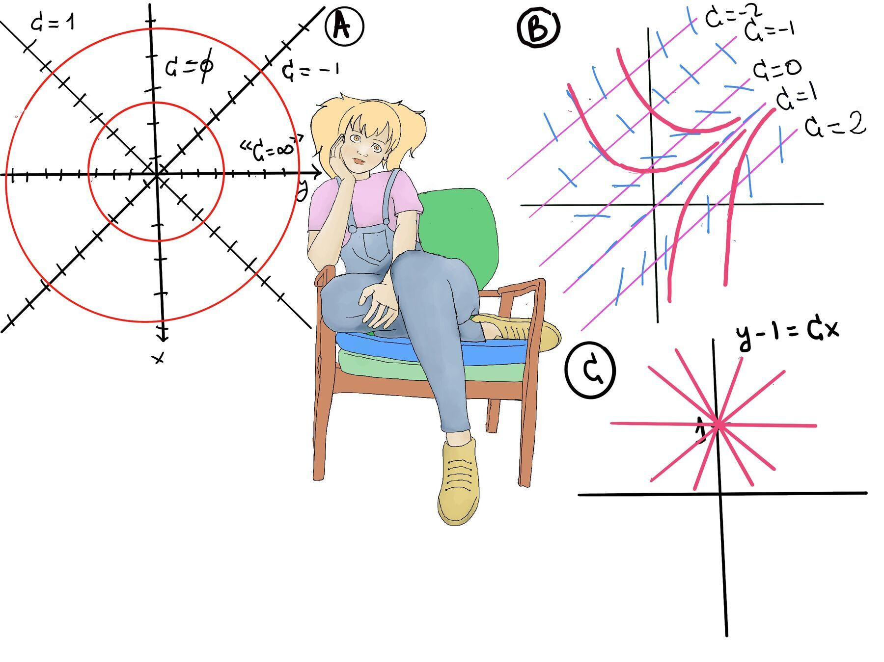
The geometric interpretation of first-order ODEs, especially using direction fields and isoclines, provides a valuable tool for visualizing and understanding the behavior of solutions. By plotting the direction field, we can see how the solution curves evolve and get a sense of the qualitative behavior of the ODE, even when an explicit solution is difficult or impossible to find.

Step 3: Analytical Verification

Given the differential equation: $y' = \frac{-x}{y}↭[\text{This can be written as:}] \frac{dy}{dx} = \frac{-x}{y}$

Separation of variables: ydy = -xdx.

Now, we can integrate both sides: $\int ydy = \int -xdx ⇒[\text{This yields:}] \frac{y^2}{2} = \frac{-x^2}{2} + C$ where C is the constant of integration. Multiply both sides by 2 to eliminate the fractions: $y^2 = -x^2 + 2C ↭ x^2 + y^2 = 2C$. This is the equation of a circle centered at the origin with radius $\sqrt{2C}$.

For simplicity, let rename the constant C as $\frac{C_1^2}{2}$, so the equation becomes: $x^2+y^2 = C_1^2$. Thus, the general solution to the ODE is: $y = \sqrt{C_1^2-x^2}$. The complete family of solutions includes both the positive and negative square roots: $y = ±\sqrt{C_1^2-x^2}$

These curves represent circles centered at the origin, as anticipated from the geometric interpretation.

Worked Example 2: Convergence and Asymptotes

Let’s examine the differential equation y’ = 1 + x - y. This is a first-order ordinary differential equation where the slope (y′) depends on both x and y. Because the slope changes depending on our coordinates, we can visualize the behavior of the solutions across the entire xy-plane using a direction field.

Step 1: Find the Isoclines and Direction Field

The direction field for a differential equation is a graphical representation that helps us visualize the behavior of solutions without explicitly solving the ODE. In a direction field:

• For each point (x, y) on the plane, we calculate the slope y’ and draw a small line segment with that exact slope.
• Collectively, these segments illustrate or suggest how solution curves flow across the plane, (refer to Figure B for a visual representation and aid in understanding it).

For the equation y′ = 1 +x −y, let’s calculate the slopes y′ at various points and draw small line segments to represent these slopes. This process, if done for many points, will yield a direction field that visually illustrates potential solution curves.

An isocline is a curve along which the slope of the direction field y’ is constant. To find the isoclines for our equation, we set the slope equal to a constant C: y’ = C.

Substituting our differential equation, the family of isoclines is given by: 1 + x -y = C or y = x + (1 - C). This represents a family of straight, parallel lines, all with a slope of 1. Each line corresponds to a different constant slope value of C in the direction field and helps us organize and understand the direction field.

Examples of Isoclines. Here are some specific values for C that help illustrate how the direction field behaves along these isoclines:

• For C = 0, we have the line y = x + 1, meaning that on this line, the direction field has a constant slope of y’ = 0, i.e., the line segments along this line are horizontal.
• For C = -1, we get the line y = x + 2, meaning that on this line the direction field has a constant slope -1, indicating line segments slanting downward at a 45° angle.
• For C = 1, this yields y = x. The slope of the direction field along this line is exactly 1 (segments slanting upward at 45°).
• For C = 2, we obtain y = x -1, with a slope of y’ = 2, meaning the line segments are even steeper and slanting upward.

Step 2: Geometric Observations (The “Corridor” Effect)

If we look between the isoclines corresponding to C = 0 and C = 2, we observe that the integral curves (solution curves) cannot escape or are confined within a corridor of isoclines unable to cross certain boundaries. All solutions in this region asymptotically approach the line y = x as x → ∞. This line y = x acts as an attractor for solutions in this region.

1. The line y = x is indeed a solution to the differential equation. If we substitute y = x into the original differential equation, we get $y' = 1 + x -y \implies 1 = 1 + x -x$. This means if a solution ever lands on the line y = x, it will stay on that line forever.
2. The Funneling Behavior:
   Above the corridor (y > x + 1): Here, C < 0. The slope segments point downward. If you drop a point here, the solution curve is forced down toward the corridor.
   Inside the upper corridor (x < y < x + 1): Here, the slopes are between 0 and 1. Because the slope of the solution is less than 1 (the slope of our asymptote), the solution grows slower than the line y = x, pulling it closer and closer to y = x.
   Inside the lower corridor (x − 1 < y < x): In this specific band, the constant C (the slope) is between 1 and 2. Because the solution’s slope is slightly greater than 1 (which is the slope of our asymptote y = x), the solution curve rises just fast enough to slowly catch up to the asymptote from below, without overshooting it.
   Below the corridor (y < x − 1): Down here, C > 2. The slope segments are very steep. Any solution starting in this region will shoot upward aggressively until it crosses the y = x −1 boundary. Once it crosses into the “lower corridor,” its slope mellows out, and it smoothly glides toward y = x.

This creates a definitive funneling effect: regardless of their starting coordinates, all solution curves eventually converge and approach the asymptote y = x as x→∞.

Bibliography

1. NPTEL-NOC IITM, Introduction to Galois Theory.
2. Algebra, Second Edition, by Michael Artin.
3. LibreTexts, Calculus and Calculus 3e (Apex). Abstract and Geometric Algebra, Abstract Algebra: Theory and Applications (Judson).
4. Field and Galois Theory, by Patrick Morandi. Springer.
5. Michael Penn, and MathMajor.
6. Contemporary Abstract Algebra, Joseph, A. Gallian.
7. YouTube’s Andrew Misseldine: Calculus. College Algebra and Abstract Algebra.
8. MIT OpenCourseWare [18.03 Differential Equations, Spring 2006], YouTube by MIT OpenCourseWare.
9. Calculus Early Transcendentals: Differential & Multi-Variable Calculus for Social Sciences.