
|
 |

|
|
|
|
|
|
There are two ways to do great mathematics. The first is to be smarter than everybody else. The second way is to be stupider than everybody else — but persistent, Raoul Bott

In this discussion, we aim to solve a system of linear differential equations of the form: $\vec{x'} = A\vec{x}$ where A is a constant 2 x 2 matrix, and $\vec{x} = (\begin{smallmatrix}x(t)\\\ y(t)\end{smallmatrix})$ is the vector of unknown functions x(t) and y(t).
The goal is to simplify the problem so that we can solve it more easily. One useful technique is to perform a change of variables, defining new variables u(t) and v(t) as linear combinations of x(t) and y(y). If chosen intelligently, these new variables can decouples the system, simplifying it into two separate (independent) first-order equations that are much easier to solve.
By making a clever choice of new variables $u(t)$ and $v(t)$, we can rewrite the system so that $u'(t)$ depends only on $u(t)$, and $v'(t)$ depends only on $v(t)$. In other words, we get $\begin{cases} u'=k_1u \\\ v'=k_2v \end{cases}$ where $k_1$ and $k_2$ are constants. These are now two simple, well-known Ordinary Differential Equations (ODEs) with standard exponential solutions.
To decouple the system, we typically introduce new variables u(t) and v(t) defined by linear combinations of x(t) and y(t):
$\begin{cases} u = ax + by \\\\ v = cx + dy \end{cases}$
The problem or core challenge is to find new variables u and v that transform the system into a decoupled form, meaning that the equations for u and v are independent of each other.
Note: In linear algebra, this “clever choice” of constants (a, b, c, d) is not just guesswork; it is directly derived from finding the eigenvectors of matrix A to diagonalize the system!
The new system should look like:
$\begin{cases} u' = k_1u \\\\ v' = k_2v \end{cases}$
where $k_1$ and $k_2$ are constants (which will turn out to be the eigenvalues of the matrix). This decoupled system consists of two separate first-order differential equations, which can be solved independently. Once we solve for $u(t)$ and $v(t)$, we can use algebraic substitution to express the original variables $x(t)$ and $y(t)$ in terms of $u(t)$ and $v(t)$.
Consider an old ice cube tray with two compartments connected by a small opening that allows liquid to flow between them. Let x(t) and y(t) represent the height of the liquid in the first and second chamber at time t, respectively. Refer to Figure i for a visual representation and aid in understanding it.
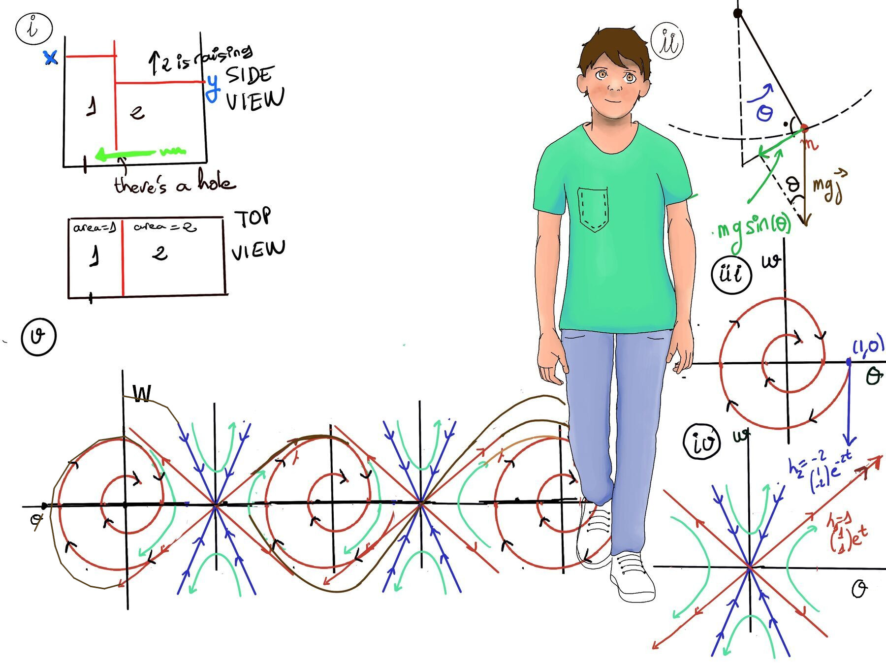
Imagine that the system evolves over time according to certain flow dynamics. The flow rate (cm/sec) between the two compartments is proportional to the pressure difference, which is related to the liquid height difference between the two chambers. We assume that the bases area of the second chamber is double that of the first.
The system is governed by the following differential equations that describe the flow of liquid:
$\begin{cases} x' = c(y-x) \\\\ 2y' = c(x-y) \end{cases}$
where:
To make the problem more simple and manageable, let’s assume c = 2. This simplifies the system to:
$\begin{cases} x' = -2x + 2y \\\\ 2y' = 2x -2y \end{cases}$
We can further simplify the second equation by dividing it by 2:
$\begin{cases} x' = -2x + 2y \\\\ y' = x -y \end{cases}$
We seek variables that can help us understand the system’s behavior and decouple it physically.
To find the dynamics of u(t), differentiate it with respect to time: $u' = x' + 2y' = (-2x + 2y) + 2(x - y) = -2x + 2y + 2x - 2y = 0$
Thus, we find that: u’(t) = 0. This confirms that u(t) is constant over time. This aligns with the conservation of mass.
Solution for $u$: $u(t) = c_1$, where $c_1$ is a constant determined by the initial total volume
Next, differentiate v(t) with respect to time: $v' = x' - y' = (-2x + 2y) - (x - y) = -2x + 2y - x + y = -3x + 3y = -3(x - y)$
Since $v = x - y$, we substitute $v$ back in to get: $v'(t) = -3v(t)$.
This is just a standard first-order linear ODE and the solution is: $v(t) = c_2 e^{-3t}$, where $c_2$ is a constant determined by the initial height difference.
We have successfully decoupled the system into two independent equations:
$\begin{cases} u' = 0 \\\\ v' = -3v \end{cases}$
The solution are: $u(t) = c_1, v(t) = c_2 e^{-3t}$
Now we must convert our solutions for $u$ and $v$ back into our original physical variables $x$ and $y$ using our system of substitutions:
$\begin{cases} u = x + 2y ~(i) \\\\ v=x−y ~(ii) \end{cases}$
From equation (ii): $v = x -y \implies[\text{Solve for }x] x = v + y$
Now substitute x = v +y into Equation (i): $u = (v+y) +2y \implies[\text{This simplifies to:}] u = v + 3y$
Solve for y: $y = \frac{u-v}{3}$
Now, that we have $y = \frac{u-v}{3}$, substitute this back into the expression for x, $x = v + y = v + \frac{u-v}{3} = \frac{u+2v}{3}$
Finally, substitute our explicit time-dependent solutions $u = c_1$ and $v = c_2 e^{-3t}$ into these equations: $x(t) = \frac{1}{3}(u+2v) = \frac{1}{3}(c_1+2c_2e^{-3t}), y = \frac{1}{3}(u-v) = \frac{1}{3}(c_1-c_2e^{-3t})$
Writing this in matrix/vector form yields our general solution: $\boxed{\vec{x} = \frac{1}{3}c_1(\begin{smallmatrix}1\\\ 1\end{smallmatrix})+ \frac{1}{3}c_2(\begin{smallmatrix}2\\\ -1\end{smallmatrix})e^{-3t}}$
The Steady-State Solution: The first term $\frac{1}{3}c_1(\begin{smallmatrix}1\\\ 1\end{smallmatrix})$ has no time-dependent exponential. It does not decay or change over time. It represents the steady-state equilibrium where the heights x(t) and y(t) are constant over time, meaning both compartments settle at a constant height radio (specifically, they reach the exact same height, a 1:1 ratio). The constant $c_1$ is determined by by the total (and initial) volume of liquid poured into the tray. Over a long time, as $t \to \infty$ the entire system converges to this steady state.
The Transient Solution: The second Term $\frac{1}{3}c_2(\begin{smallmatrix}2\\\ -1\end{smallmatrix})e^{-3t}$ represents the transient behavior caused by the initial height difference between the compartments and describes how these differences dissipate over time The exponential factor $e^{-3t}$ acts as a damping decay, meaning any initial imbalance in the heights rapidly vanishes, driving the system to equilibrium.
We aim to solve a system of linear differential equations of the form: $\vec{x'} = A\vec{x}$ where A is a constant 2 x 2 matrix, and $\vec{x} = (\begin{smallmatrix}x(t)\\\ y(t)\end{smallmatrix})$ is the vector of unknown functions x(t) and y(t).
We seek a transformation of variables that “decouples” this system, transforming it into two independent equations that can be solved separately. This approach simplifies the problem significantly. After decoupling, we ideally want a system of the form:
$\begin{cases} u' = \lambda_1 u \\ v' = \lambda_2 v \end{cases}$
where $u(t)$ and $v(t)$ are new variables that describe the system, and $\lambda_1$ and $\lambda_2$ are the eigenvalues of matrix $A$.
For a 2 × 2 matrix A, the standard method to decouple the system $\vec{x'} = A\vec{x}$ involves diagonalizing A. To do this successfully, certain conditions must be met:
Let E be the matrix whose columns are the eigenvectors of A: $E = (\vec{α_1}~\vec{α_2}) = (\begin{smallmatrix}a_1 & a_2\\\ b_1 & b_2\end{smallmatrix})$
We introduce a change of variables: $\vec{x} = E\vec{u}$ where $\vec{u} = (\begin{smallmatrix}u\\\ v\end{smallmatrix})$
Differentiating both sides with respect to t: $\vec{x'} = E\vec{u'}$.
Since the original system is $\vec{x'} = A\vec{x}$, we can substitute our new definitions: $E\vec{u'}= A\vec{x} = A(E\vec{u})$
By the properties of matrix multiplication $A(Eu) = (AE)u$. We can substitute AE = ED [🚀] where D is the diagonal matrix of eigenvalues ($D = (\begin{smallmatrix}\lambda_1 & 0\\\ 0 & \lambda_2\end{smallmatrix})$). This transforms our equation to: $E\vec{u'}= A(E\vec{u}) = (AE)\vec{u} = ED\vec{u} ↭ E\vec{u'}= ED\vec{u}$
[🚀] Proof that AE = ED.
Using the definition of eigenvectors, $(A - \lambda I)\vec{\alpha} = \vec{0} \implies A\vec{\alpha} = \lambda\vec{\alpha}$
Therefore, for each column: $AE = A(\vec{α_1}\;\vec{α_2}) = (A\vec{α_1}\;A\vec{α_2})= (λ_1\vec{α_1}\;λ_2\vec{α_2})$
Multiplying the eigenvector matrix by the diagonal eigenvalue matrix yields the exact same scaling: $ED = (\vec{α_1}\;\vec{α_2})(\begin{smallmatrix}λ_1 & 0\\\ 0 & λ_2\end{smallmatrix}) = (λ_1\vec{α_1}\;λ_2\vec{α_2})$.
Since both sides yield the same result, we have: AE = ED.
Going back, we simplify the equation $E\vec{u}' = ED\vec{u}$ by multiplying both sides on the left by $E^{-1}$: $E^{-1}E\vec{u'}= E^{-1}ED\vec{u} ⇒ \vec{u'} = D\vec{u}$
Since D is diagonal, this results in the perfectly decoupled system:
$\begin{cases} u' = λ_1u \\\ v' = λ_2v \end{cases}$.
The decoupled equations can now be solved independently as standard first-order linear ODEs:
where $c_1$ and $c_2$ are constants determined by the initial conditions of the system.
To find the solution in terms of our original variables, we use the initial transformation $\vec{x} = E\vec{u}$: $\vec{x} = E\vec{u} = (\vec{α_1}\;\vec{α_2})(\begin{smallmatrix}u(t)\\\ v(t)\end{smallmatrix}) = (\vec{α_1}\;\vec{α_2})(\begin{smallmatrix}c_1e^{λ_1t}\\\ c_2e^{λ_2t}\end{smallmatrix}) = c_1e^{λ_1t}\vec{α_1} + c_2e^{λ_2t}\vec{α_2}$
Therefore, the general solution to the original system is simply a linear combination of the eigenvectors scaled by their respective exponential eigenvalues: $\vec{x}(t) = c_1 e^{\lambda_1 t}\vec{\alpha_1} + c_2 e^{\lambda_2 t}\vec{\alpha_2}$.
Let’s solve the following system of differential equations by transforming it into a decoupled system where each equation involves only one of the new variables. This makes solving the system straightforward.
$\begin{cases} x' = -2x + 2y \\\\ y' = x -y \end{cases}$
Step 1: Writing the System in Matrix Form
We can express the system in matrix form as: $\vec{x'} = A\vec{x}$ where A = $(\begin{smallmatrix}-2 & 2\\\ 1 & -1\end{smallmatrix})$, $\vec{x} = (\begin{smallmatrix}x\\\ y\end{smallmatrix})$
$(\begin{smallmatrix}x'\\\ y'\end{smallmatrix}) = (\begin{smallmatrix}-2 & 2\\\ 1 & -1\end{smallmatrix})(\begin{smallmatrix}x\\\ y\end{smallmatrix})$
Step 2: Find Eigenvalues of A
The eigenvalues ($\lambda$) of matrix A are found by solving the characteristic equation: $\det(A - \lambda I) = 0$ where I is the identity matrix.
Compute $\det \begin{pmatrix} -2-\lambda & 2 \\ 1 & -1-\lambda \end{pmatrix} = (-2-\lambda)(-1-\lambda) - (2)(1) = 0$
$(2 + 3\lambda + \lambda^2) - 2 = 0 \implies \lambda^2 + 3\lambda = 0$
Factoring out $\lambda$ gives $\lambda(\lambda + 3) = 0$, yielding solutions: $\lambda_1 = 0$ and $\lambda_2 = -3$.
Step 3. Find Eigenvectors
This yields $a_1 - b_1 = 0 \implies a_1 = b_1$. Choosing $1$ for simplicity gives $\vec{\alpha_1} = \begin{pmatrix} 1 \\ 1 \end{pmatrix}$.
This yields $a_2 + 2b_2 = 0 \implies a_2 = -2b_2$. Choosing $b_2 = 1$ gives $\vec{\alpha_2} = \begin{pmatrix} -2 \\ 1 \end{pmatrix}$.
Step 4: Constructing the Matrix E and its inverse
The matrix E is formed by placing the eigenvectors as columns: E = $(\vec{α_1}\;\vec{α_2}) = (\begin{smallmatrix}1 & -2\\\ 1 & 1\end{smallmatrix})$
Since we have two linearly independent eigenvectors, A is diagonalizable. Nowe, we compute $E^{-1}$: det(E) = $det(\begin{smallmatrix}1 & -2\\\ 1 & 1\end{smallmatrix}) = 1·1−(−2)·1 = 1+2 =3.$
Then, $E^{-1} = \frac{1}{det(E)}·(\begin{smallmatrix}e_{22} & -e_{12}\\\ -e_{21} & e_{11}\end{smallmatrix})= \frac{1}{3}(\begin{smallmatrix}1 & 2\\\ -1 & 1\end{smallmatrix})$
Step 5: Define the Change of Variables
We introduce the decoupled variables: $\vec{u} = E^{-1}\vec{x} = \frac{1}{3}(\begin{smallmatrix}1 & 2\\\ -1 & 1\end{smallmatrix})(\begin{smallmatrix}x\\\ y\end{smallmatrix}) = (\begin{smallmatrix}u\\\ v\end{smallmatrix})$
Thus, the specific transformation is: u = $\frac{1}{3}(x+2y)$, v = $\frac{1}{3}(-x+y)$
Conversely, expressing $\vec{x}$ in Terms of $\vec{u}$: $\vec{x} = E\vec{u} = (\begin{smallmatrix}1 & -2\\\ 1 & 1\end{smallmatrix})(\begin{smallmatrix}u\\\ v\end{smallmatrix})$. This results in: $x = u −2v, y = u +v$.
Step 6: Transform and Solve the Decoupled System
Substituting into $E\vec{u'} = ED\vec{u}$ yields: $\begin{pmatrix} u' \\ v' \end{pmatrix} = \begin{pmatrix} 0 & 0 \\ 0 & -3 \end{pmatrix} \begin{pmatrix} u \\ v \end{pmatrix}$ where $\lambda_1 = 0, \lambda_2 = -3$.
This separates neatly into: $\begin{cases} u' = 0 \implies u(t) = c_1 \\ v' = -3v \implies v(t) = c_2 e^{-3t} \end{cases}$
Step 7: Write the Final General Solution
Substitute the solutions for $u(t)$ and $v(t)$ back into our original variable relationships ($x = u - 2v$, $y = u + v$): $x(t) = c_1 - 2c_2 e^{-3t}$, $y(t) = c_1 + c_2 e^{-3t}$
Written cleanly as a vector: $\boxed{\vec{x}(t) = \begin{pmatrix} x(t) \\ y(t) \end{pmatrix} = c_1 \begin{pmatrix} 1 \\ 1 \end{pmatrix} + c_2 e^{-3t} \begin{pmatrix} -2 \\ 1 \end{pmatrix}}$
Interpretation:

JustToThePoint Copyright © 2011 - 2026 Anawim. ALL RIGHTS RESERVED. Bilingual e-books, articles, and videos to help your child and your entire family succeed, develop a healthy lifestyle, and have a lot of fun. Social Issues, Join us.
This website uses cookies to improve your navigation experience.
By continuing, you are consenting to our
use of cookies, in accordance with our Cookies Policy and
Website Terms and Conditions of use.