
|
 |

|
|
|
|
|
|
The scariest monsters are the ones that lurk within our souls, Edgar Allen Poe.

Convolution is a powerful mathematical operation that blends two functions together to produce a third function. It is widely used in engineering, physics, signal processing, and applied mathematics to analyze systems and solve differential equations.
The convolution of two functions $f(t)$ and $g(t)$ is denoted by $(f * g)(t)$ and is defined by the integral $\boxed{(f * g)(t) = \int_{0}^{t} f(u)g(t-u) du}$

In the study of differential equations and physical systems, impulse inputs represent sudden forces applied over a very short period of time. These impulses model events like a hammer strike, a bat hitting a baseball, a collision, a sudden voltage spike in a circuit, or any scenario where a large force is exerted briefly. Understanding how to model and analyze these impulses is crucial for accurately describing and predicting how physical systems respond to sudden shocks.
If a force $f(t)$ is applied over a specific time interval $[a, b]$, the impulse delivered over that interval is defined as the integral of the force over time: $\boxed{\text{Impulse} = \int_{a}^{b} f(t) dt}$
Physical Intuition: The impulse represents the total effect of a force applied over a time interval, accounting for both its magnitude and its duration. It has units of force multiplied by time (e.g., Newton-seconds). Physically, impulse is equal to the change in momentum of the object.
In the simple case where $f(t)$ is a constant force $F$, the impulse simplifies to the area of a rectangle: $\text{Impulse} = \int_{a}^{b} F \, dt = F \cdot (b-a)$. The total impulse is proportional to the magnitude of the force and the duration over which it is applied. It is simply the area under the force-time graph between t = a and t = b.
To model a sudden hammer strike mathematically, we can represent the force using a “box function.” This function is zero everywhere, except over a tiny time interval $[0, h]$ where it exerts a constant force.
Let’s imagine applying a short burst of force to a mass. We want to deliver a Unit Impulse (an impulse with a total area of exactly $1$).
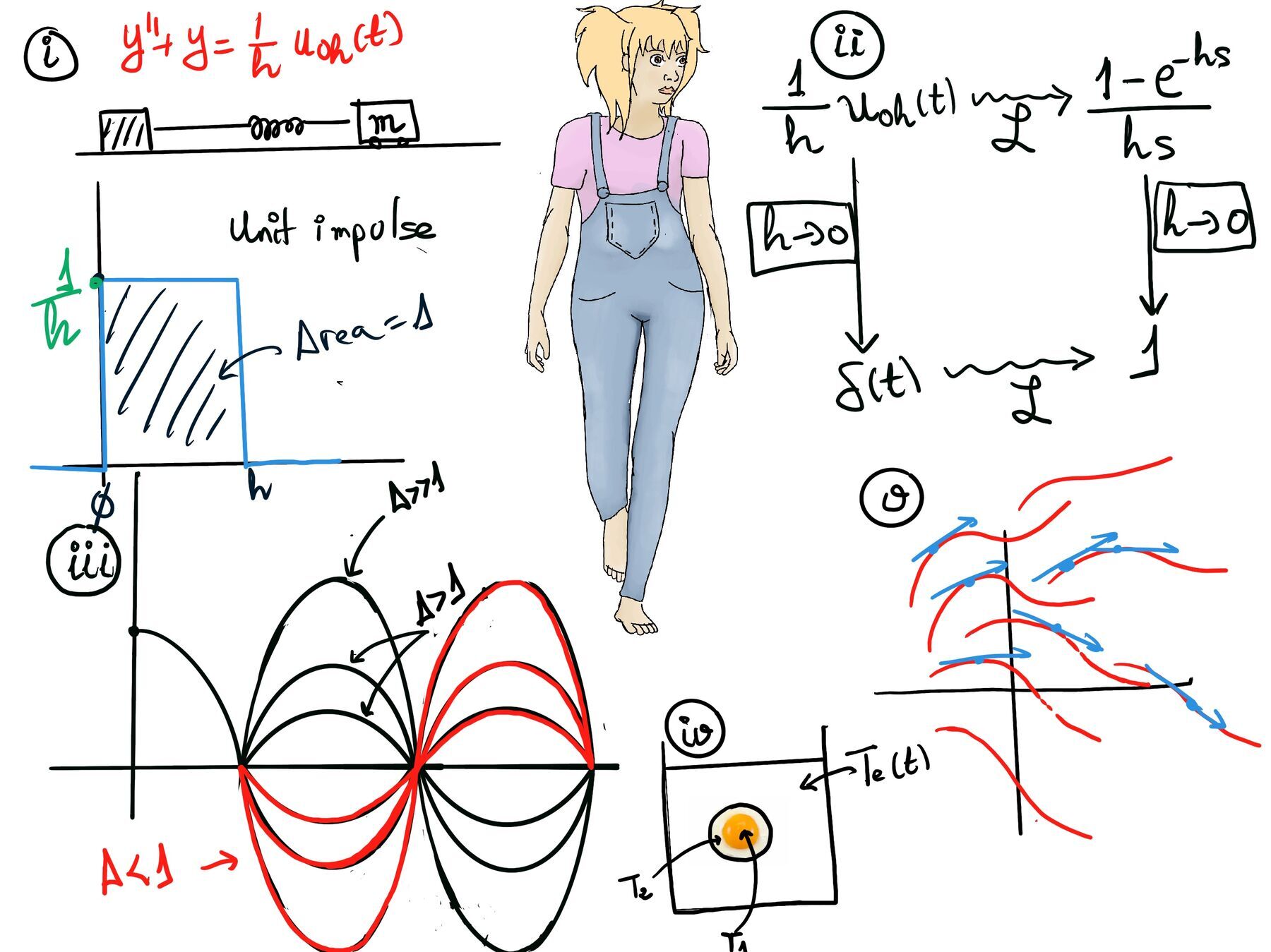
As the time interval $h$ becomes shorter and shorter, the magnitude of the force ($\frac{1}{h}$) must increase to maintain a constant total area of $1$. This reflects the idea that an impulse is a very large force applied over an infinitesimally small time period.
Consider an undamped mass-spring system with mass m. When an impulse is applied, such as a sudden push or hit, we can model the force over a small time interval, say [0, h], e.g., image applying a short burst of force to the mass over this brief period (Refer to Figure i for a visual representation and aid in understanding it), by using a box function.
Using the Heaviside step function $u(t)$, we define this “unit impulse box function” $f_h(t)$ as: $\boxed{f_h(t) = \frac{1}{h}[u(t) - u(t-h)]}$
Let’s verify its total impulse (area): $\text{Impulse} = \int_{0}^{\infty} f_h(t) dt = \int_{0}^{h} \frac{1}{h} dt = \left[ \frac{t}{h} \right]_{0}^{h} = \frac{h}{h} = 1$
Let’s apply this to a real system. The equation of motion for the undamped mass-spring system under the action of the impulse is: $my'' + ky = F_{\text{ext}}(t)$
For simplicity, let mass $m = 1$ and spring constant $k = 1$. Let our external force be the unit impulse box function $f_h(t)$: $y'' + y = \frac{1}{h}[u(t) - u(t-h)]$ where:
To solve the differential equation, we apply the Laplace Transform, which converts differential equations into algebraic equations in the s-domain.
Laplace Transform of the Forcing Function.
Recall the Laplace Transform of a step function: $u(t) \leadsto \frac{1}{s}, u(t-a) \leadsto e^{-as}\frac{1}{s}$
Applying this to our box function (where $a=0$ and $a=h$): $\mathcal{L}\{f_h(t)\} = \frac{1}{h} \left[ \frac{1}{s} - \frac{e^{-hs}}{s} \right] = \frac{1 - e^{-hs}}{hs}$
This rational expression represents the Laplace Transform of the physical hammer strike.
Take the Limit as $h \to 0$.
A true instantaneous impulse means the time interval $h$ approaches exactly zero.
Let’s see what happens to our Laplace transform as $h \to 0$: $\lim_{h \to 0} \mathcal{L}\{f_h(t)\} = \lim_{h \to 0} \frac{1 - e^{-hs}}{hs}$
Because plugging in $h=0$ gives the indeterminate form $\frac{0}{0}$, we apply L’Hôpital’s Rule.
We differentiate the numerator and denominator with respect to $h$ (treating $s$ as a constant):
Derivative of numerator w.r.t $h$: $0 - (-s)e^{-hs} = s e^{-hs}$
Derivative of denominator w.r.t $h$: $s$
$= \lim_{h \to 0} \frac{s e^{-hs}}{s} = \lim_{h \to 0} e^{-hs} = e^0 = 1$
On the physical side, as $h \to 0$, the time interval becomes infinitely small, and the force magnitude goes to infinity. The box function $f_h(t)$ collapses into a purely theoretical mathematical construct known as the Dirac Delta function, denoted by $\delta(t)$.
The Dirac delta function $\delta(t)$, also known as the unit impulse, is not a function in the traditional sense but a mathematical construct that models an impulse occurring at a single point in time. It is a generalized function on the real numbers or distribution, whose value is zero everywhere except at zero t = 0, and whose integral over the entire real line is equal to one
Conclusion: Because the limit of the box function’s transform is $1$, the Laplace Transform of the ideal Dirac Delta function is exactly: $\boxed{\mathcal{L}\{\delta(t)\} = 1}$
The Dirac Delta $\delta(t)$ is a distribution or generalized function. It is defined conceptually as: $\delta(t) = \begin{cases} \infty, & t = 0 \\ 0, & t \neq 0 \end{cases}$
It acts as an infinitely high, infinitely narrow spike at $t=0$, but it maintains a perfect area of $1$: $\boxed{\int_{-\infty}^{\infty} \delta(t) dt = 1}$
The most important property of the Dirac delta function is the sifting property, which states that for any function g(t) that is continuos at t = a: $\int_{-∞}^{∞} \delta(t-a)g(t)dt = g(a)$. In other words, the delta function centered a t = a “picks out” the value of g(t) at t = a.
This makes $\delta(t)$ an incredibly powerful mathematical tool. It allows us to easily inject sudden, instantaneous energy into differential equations using algebraic simplicity ($\mathcal{L}\{\delta\} = 1$) rather than dealing with messy, discontinuous integrals!
The Dirac delta function $\delta(t)$ is difficult to grasp initially because it is not a traditional function. One of the best ways to understand it is by considering it as the limit of a sequence of regular functions that become infinitely narrow and infinitely tall.
Consider a rectangular pulse approximation of the delta function centered at $t = a$. Let $\delta_{a, \varepsilon}(t)$ be a function that is zero everywhere except on a tiny interval $[a, a + \varepsilon]$, where it has a constant height of $\frac{1}{\varepsilon}$:
$$\delta_{a, \varepsilon}(t) = \begin{cases} \frac{1}{\varepsilon}, & t \in [a, a + \varepsilon] \\ 0, & \text{otherwise} \end{cases}$$where $\varepsilon > 0$ is an infinitesimally small number.
Notice that the area of this pulse is exactly $1$ ($\text{width} \times \text{height} = \varepsilon \cdot \frac{1}{\varepsilon} = 1$).
The Mean Value Theorem for Integrals states that if f(t) is continuous on the closed interval [a, b], then there exists a point $c \in [a, b]$ such that: $\int_{a}^{b} f(t)dt = (b-a)f(c)$
The total area under f(t) from a to b equals the area of a rectangle with width b − a and height f(c).
Let’s calculate: $\int_{-∞}^{∞} \delta_{a, ε}(t)g(t)dt = \int_{a}^{a+ ε} \frac{1}{ε}g(t)dt =[...]$
By the Mean Value Theorem for Integrals, since g(t) is continuous on the interval $[a, a + \varepsilon]$, there exists a point $c \in [a, b]$ such that: $\int_{a}^{a+ ε} g(t)dt = ε·g(c)$.
Substitute this back into our equation: $\int_{∞}^{-∞} δ_{a, ε}(t)g(t)dt = \int_{a}^{a+ ε} \frac{1}{ε}g(t)dt =ε·\frac{1}{ε}g(c) = g(c)$.
Now, we take the limit as the pulse becomes infinitely narrow $\varepsilon \to 0$, the interval [a, a+ε] shrinks to a single point t = a, and since g(t) is continuous at t = a, $g(c) \to g(a)$, hence $\lim_{ε \to 0} \int_{∞}^{-∞} δ_{a, ε}(t)g(t)dt \to g(a)$.
Therefore, the sifting property holds: $\int_{∞}^{-∞} δ_a(t)g(t)dt = g(a)$ The integral effectively “samples” the exact value of the function at the location of the impulse!
Special Case: a = 0, the Dirac delta function becomes $\delta(t)$, centered at the origin. Thus, for any continuous function f(t): $\int_{-∞}^{∞} \delta(t)f(t)dt = f(0)$
An incredibly important property of the delta function is its relationship with the unit step function $u(t)$.
If you take the derivative of the step function $u(t-a)$, it is $0$ everywhere except at $t=a$, where it jumps vertically from $0$ to $1$ in zero time, resulting in an infinite slope. Thus, the derivative of the unit step function is the delta function: $\boxed{\frac{d}{dt} u(t-a) = \delta(t-a)}$ (the derivative captures this instantaneous and abrupt change as the Dirac delta function at t = a.)
Using the sifting property, finding the Laplace Transform of an impulse is incredibly simple. It just picks out the value of $f(t) = e^{-st}$ at the moment the impulse fires!
Delayed Impulse at $t = a$: $\mathcal{L}\{\delta(t-a)\} = \int_{0}^{\infty} e^{-st}\delta(t-a) dt = e^{-as}$
💡 This makes the delta function a powerful tool in modeling instantaneous forces or idealized impulses, as it encapsulates the idea of applying a force over an infinitesimally small time period (a force that acts instantaneously at t = 0 or a, e.g., if you strike a mass-spring system with a hammer), while still imparting a finite impulse. It completely eliminates the complexity of the $s$-domain variable (turning it into a constant $1$), allowing us to easily inject sudden, idealized forces into a system.
In the context of the Laplace Transform, we typically deal with causal functions —functions that are defined as zero for t < 0.
Next, we explore how the delta function behaves under convolution.
Let f be an arbitrary function. The convolution of f(t) with the delta function $\delta(t)$ is defined as: $(f * \delta)(t) = \int_{0}^{t} f(\tau)\delta(t - \tau) d\tau$
Since $\delta(t - \tau)$ is a spike that fires exactly when $\tau = t$, the integral simply reduces to f(t) (it sifts out the value of $f(\tau)$ at $\tau = t$).
This perfectly matches the logic of the Laplace domain. By the Convolution Theorem, convolution in time is multiplication in frequency. Since $\mathcal{L}\{\delta(t)\} = 1$, $\mathcal{L}\{(f * \delta)(t)\} = F(s) \cdot 1 = F(s)$
$u(t)f(t) * δ(t) \leadsto_{\mathcal{L}} F(s)·1, u(t)f(t)\leadsto_{\mathcal{L}} F(s)$. Therefore, $u(t)f(t) * δ(t) = u(t)f(t)$. The delta function acts as the identity element under convolution. In other words, convolving any function with δ(t) simply reproduces the original function. This property reflects the nature of the delta function as a mathematical “impulse” that isolates the behavior of a system at a specific moment in time.
Additionally, the derivative of the step function u(t) is the delta function: $u'(t) = \delta(t)$.
The step function jumps from 0 to 1 at t = 0, and its derivative is the delta function at that point.

JustToThePoint Copyright © 2011 - 2026 Anawim. ALL RIGHTS RESERVED. Bilingual e-books, articles, and videos to help your child and your entire family succeed, develop a healthy lifestyle, and have a lot of fun. Social Issues, Join us.
This website uses cookies to improve your navigation experience.
By continuing, you are consenting to our
use of cookies, in accordance with our Cookies Policy and
Website Terms and Conditions of use.