
|
 |

|
|
|
|
|
|
The scariest monsters are the ones that lurk within our souls, Edgar Allen Poe.

The Laplace Transform of a function f(t), where t ≥ 0, is defined as $\mathcal{L}(f(t)) = \int_{0}^{∞} f(t)e^{-st}dt = F(s)$.
One of the most important properties of the Laplace Transform is linearity, which states: $\mathcal{L}(af(t)+bg(t)) = a\mathcal{L}(f(t))+b\mathcal{L}(g(t))$
The following table summarizes the most frequent mappings used in system analysis.
| Function | Laplace Transform |
|---|---|
| Unit Step, u(t) | $\mathcal{L}(u(t)) = \frac{1}{s}, s > 0$ |
| Exponential, $e^{at}$ | $\frac{1}{s - a}, s > a$ |
| Complex Exp $e^{(a + bi)t}$ | $\mathcal{L}(e^{(a + bi)t}) = \frac{1}{s - (a + bi)}, s > a$ |
| Cosine $\cos(\omega t)$ | $\mathcal{L}(\cos(\omega t)) = \frac{s}{s^2 + \omega^2}, s > 0$ |
| Sine $\sin(\omega t)$ | $\mathcal{L}(\sin(\omega t)) = \frac{\omega}{s^2 + \omega^2}, s > 0$ |
| Power, $t^n$ | $\mathcal{L}(t^n) = \frac{n!}{s^{n+1}}, s > 0$ |
| Delayed Step, $u(t-a)$ | $\mathcal{L}(u(t-a)) = \frac{e^{-as}}{s}, s > 0$ |
| Dirac Delta $\delta(t-a)$ | $\mathcal{L}(\delta(t-a)) = e^{-as}, a \geq 0$ |
| $\frac{1}{t}$ | $\mathcal{L}\left(\frac{1}{t}\right) = \text{not defined}$ |
| $e^{-bt} \cos(\omega t)$ | $\mathcal{L}(e^{-bt} \cos(\omega t)) = \frac{s + b}{(s + b)^2 + \omega^2}, s > -b$ |
| $e^{-bt} \sin(\omega t)$ | $\mathcal{L}(e^{-bt} \sin(\omega t)) = \frac{\omega}{(s + b)^2 + \omega^2}, s > -b$ |
| $e^{at}f(t)$ | $\mathcal{L}(e^{at}f(t)) = F(s-a)$ |

Convolution is a powerful mathematical operation that blends two functions together to produce a third function. It is widely used in engineering, physics, signal processing, and applied mathematics to analyze systems and solve differential equations.
The convolution of two functions $f(t)$ and $g(t)$ is denoted by $(f * g)(t)$ and is defined by the integral $\boxed{(f * g)(t) = \int_{0}^{t} f(u)g(t-u) du}$
Think of convolution as a “Flip, Shift, Multiply, and Integrate” operation:
Given two functions $f(t)$ and $g(t)$, their individual Laplace Transforms are: $F(s) = \mathcal{L}\{f(t)\} = \int_{0}^{\infty} f(t)e^{-st} dt$ and $G(s) = \mathcal{L}\{g(t)\} = \int_{0}^{\infty} g(t)e^{-st} dt$ respectively.
A common, intuitive assumption is that the Laplace Transform of a product, $f(t) \cdot g(t)$, would just be $F(s) \cdot G(s)$. This is false. There is no direct, simple formula for the Laplace Transform of the product $\mathcal{L}{f(t) \cdot g(t)} in terms of their individual Laplace Transforms?
However, there is an incredibly elegant relationship between the multiplication of transforms and the convolution of functions.
The Convolution Theorem states that the Laplace Transform of the convolution of two functions f(t) and g(t) in the time domain, denoted as $(f * g)(t)$, is equal to the product of their individual Laplace transforms in the frequency domain. Mathematically, $\mathcal{L}((f * g)(t)) = F(s)G(s) ↭ F(s)G(s) = \int_{0}^{∞} e^{-st}(f*g)(t)dt$ where F(s) is the Laplace transform of f(t) and G(s) is the Laplace transform of g(t).
This theorem provides a massive shortcut. It means that instead of evaluating a “cruel” convolution integral in the time domain, we can simply translate our functions to the $s$-domain, multiply them algebraically, and take the inverse transform.
Proof.
We want to prove that $F(s)G(s) = \int_{0}^{\infty} e^{-st}(f * g)(t) dt$.
Step 1: Set up the product of the transforms
Using two different dummy variables ($u$ and $v$) to avoid confusion, we multiply the definitions of $F(s)$ and $G(s)$: $F(s)G(s) = \left( \int_{0}^{\infty} f(u)e^{-su} du \right) \left( \int_{0}^{\infty} g(v)e^{-sv} dv \right)$
Combine them into a double integral over the first quadrant of the $uv$-plane ($u \ge 0, v \ge 0$): $F(s)G(s) = \int_{0}^{\infty} \int_{0}^{\infty} f(u)g(v) e^{-s(u+v)} du \, dv$
Step 2: Change of Variables
We want to introduce $t$. Let $t = u + v$. This means $v = t - u$. We will keep $u = u$.
To change the differential $du \, dv$ to $du \, dt$, we must compute the Jacobian determinant of the transformation: $|J| = \begin{vmatrix} \frac{\partial u}{\partial u} & \frac{\partial u}{\partial t} \\ \frac{\partial v}{\partial u} & \frac{\partial v}{\partial t} \end{vmatrix} = \begin{vmatrix} 1 & 0 \\ -1 & 1 \end{vmatrix} = (1)(1) - (0)(-1) = 1$
Because the Jacobian is $1$, $du \, dv = du \, dt$. Hence, the differentials remain dudt because the Jacobian determinant of the transformation is 1.
Substitute $t$ and $v$ into the integral: $= \iint f(u)g(t-u)e^{-st} du \, dt$
Step 3: Determine the new limits of integration (The tricky part!)
Originally, $u$ goes from $0 \to \infty$ and $v$ goes from $0 \to \infty$.
Since $t = u + v$, and the smallest $v$ can be is $0$, the smallest $t$ can be for a given $u$ is $t = u$. Thus, $t$ ranges from $u$ to $\infty$ (Refer to Figure ii for a visual representation and aid in understanding it)
Similarly, looking at the region (a triangle bounded by $t=u$ and the $y$-axis), if we sweep $t$ from $0 \to \infty$ on the outside, then for any fixed $t$, $u$ ranges from $0$ up to $t$, $\int_{t=0}^{∞}(\int_{u=0}^{t}e^{-st}f(u)g(t-u)du)dt$. In other words, since v = t - u, the conditions $u \ge 0$ and $v \ge 0$ become $u \ge 0,\quad t - u \ge 0 \;\Rightarrow\; u \le t.$

To make this look like a Laplace transform, we must swap the order of integration (integrate with respect to $u$ first, then $t$).
Looking at the region (a triangle bounded by $t=u$ and the $y$-axis), if we sweep $t$ from $0 \to \infty$ on the outside, then for any fixed $t$, $u$ ranges from $0$ up to $t$.
$$= \int_{0}^{\infty} \left( \int_{0}^{t} f(u)g(t-u)e^{-st} du \right) dt$$Step 4: Isolate the Convolution
Pull $e^{-st}$ out of the inner integral, since it does not depend on $u$: $= \int_{0}^{\infty} e^{-st} \left[ \int_{0}^{t} f(u)g(t-u) du \right] dt$
The term in the brackets is exactly the definition of convolution $(f * g)(t)$! Therefore, $= \int_{0}^{\infty} e^{-st} (f * g)(t) dt= \mathcal{L}\{(f * g)(t)\}$ (Q.E.D)
Commutativity: $f * g = g * f$
Proof via substitution: Let $(f * g)(t) = \int_{0}^{t} f(u)g(t-u) du$.
Let $\tau = t - u \implies du = -d\tau$.
When $u=0, \tau=t$. When $u=t, \tau=0$.
Associativity: $f * (g * h) = (f * g) * h$. The convolution operation is associative, meaning that the order in which convolutions are performed does not affect the final result.
Distributivity Over Addition: $f * (g + h) = (f * g) + (f * h)$. Convolution distributes smoothly over addition.
Identity with the Delta Function: $f(t) * \delta(t) = f(t)$
Convolving a function with the Dirac delta function returns the original function (much like multiplying by 1).
The Convolution Theorem: $\mathcal{L}(f(t)*g(t)) = \mathcal{L}(f(t))·\mathcal{L}(g(t))↭ \mathcal{L}^{-1}(F(s)·G(s)) = f(t)*g(t)$
To understand how convolution works in practice, let’s solve a purely mathematical example using two different methods: the definition of the integral, and the Convolution Theorem via the Laplace Transform.
We want to find $(t^2 * t)(t)$.
Method A: Using the Convolution Integral Definition
By definition, $(f * g)(t) = \int_{0}^{t} f(u)g(t-u) du$.
Let $f(t) = t^2 \implies f(u) = u^2$. Let $g(t) = t \implies g(t-u) = (t-u)$.
Set up the integral: $(t^2 * t) = \int_{0}^{t} u^2(t-u) du = \int_{0}^{t} (u^2 t - u^3) du$
Since we are integrating with respect to $u$, $t$ acts as a constant: $= \left[ \frac{u^3}{3}t - \frac{u^4}{4} \right]_{0}^{t}$
Substitute the limits ($u=t$ and $u=0$): $= \left( \frac{t^3}{3}t - \frac{t^4}{4} \right) - (0 - 0) =[\text{Simplify}] = \frac{t^4}{3} - \frac{t^4}{4} = \frac{4t^4 - 3t^4}{12} = \frac{t^4}{12}$
Method B: Using the Laplace Transform
Take the Laplace Transform of each function: Recall the rule $\mathcal{L}\{t^n\} = \frac{n!}{s^{n+1}}$. Therefore, $F(s) = \mathcal{L}\{t^2\} = \frac{2!}{s^3} = \frac{2}{s^3}$ and $G(s) = \mathcal{L}\{t\} = \frac{1!}{s^2} = \frac{1}{s^2}$
Multiply the Laplace Transform. By the Convolution Theorem: $\mathcal{L}\{(f * g)(t)\} = F(s) \cdot G(s)$.
$F(s)G(s) = \left(\frac{2}{s^3}\right) \left(\frac{1}{s^2}\right) = \frac{2}{s^5}$
Take the Inverse Laplace Transform.
We need to find $\mathcal{L}^{-1}\left\{\frac{2}{s^5}\right\}$. We know that $\mathcal{L}\{t^4\} = \frac{4!}{s^5} = \frac{24}{s^5}$.
To match our numerator (2) with the standard form (24), we multiply and divide by 12, $\mathcal{L}^{-1}\left\{\frac{2}{s^5}\right\} = \mathcal{L}^{-1}\left\{\frac{1}{12} \cdot \frac{24}{s^5}\right\} = \frac{1}{12} \mathcal{L}^{-1}\left\{\frac{4!}{s^5}\right\} = \frac{t^4}{12}$
As it was expected, both methods yield the exact same result: $\boxed{(t^2 * t)(t) = \frac{t^4}{12}}$.
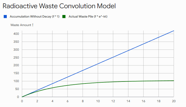
What happens if we convolve a function $f(t)$ with the constant $1$? $(f * 1)(t) = \int_{0}^{t} f(u) \cdot 1 \, du = \int_{0}^{t} f(u) du$
💡 Core Concept: Convolution with the constant function 1 results in the cumulative integral (accumulation) of $f(t)$ up to time $t$. This operation is equivalent to finding the total accumulated area under the curve (or the definite integral) of $f(t)$ from $0$ to $t$.
Convolution can be intuitively understood as a mathematical way of combining two processes: an ongoing input signal and a system’s impulse response. It calculates the current output of a system by looking at the entire history of inputs and determining how much of each past input is still affecting the present.
Imagine a factory is continuously dumping radioactive waste onto a pile over time.
Input Function $f(t)$: The rate at which new waste is added to the pile (e.g., kg per year).
System’s Response $g(t)$: The decay function of the waste over time, typically $e^{-kt}$ (where $k$ is the decay constant), representing the fraction of waste that remains after a given time.
If we want to know the total amount of radioactive waste remaining at time $t$, we must account for the fact that waste dumped yesterday has decayed a little, but waste dumped a decade ago has decayed quite a lot.
Let’s break time into tiny intervals.
At any later time t, the total amount of radioactive waste left on the pile will depend on two factors = [How much waste was dumped at each earlier time] x [How much has decayed since that earlier time].
To find the total waste currently on the pile, we sum up the remaining contributions from every single moment in the past. As we make our time intervals ($\Delta u_u$) infinitely small, this sum becomes an integral: $\text{Total Waste}(t) = \int_{0}^{t} f(u) e^{-k(t-u)} du = (f(t) * e^{-kt})$
This integral is exactly the convolution of the dumping rate $f(t)$ with the decay function $e^{-kt}$. It seamlessly combines the historical accumulation of the input with the natural decay response of the system.
Special Cases of Convolution:

JustToThePoint Copyright © 2011 - 2026 Anawim. ALL RIGHTS RESERVED. Bilingual e-books, articles, and videos to help your child and your entire family succeed, develop a healthy lifestyle, and have a lot of fun. Social Issues, Join us.
This website uses cookies to improve your navigation experience.
By continuing, you are consenting to our
use of cookies, in accordance with our Cookies Policy and
Website Terms and Conditions of use.