
|
 |

|
|
|
|
|
|

If you find yourself in a hole, stop digging, Will Rogers
Non-linear autonomous systems describe how the state of a system evolves over time when the system’s governing rules do not explicitly depend on time. By focusing on two variables x and y, we define a 2D non-linear autonomous system:
$\begin{cases} \frac{dx}{dt} = f(x, y) \quad (i) \\ \frac{dy}{dt} = g(x, y) \quad (ii) \end{cases}$
This system defines how x(t) and y(t) change with respect to time t. The functions f and g describe the system’s “velocity” in the x and y directions, respectively.
To better understand the behavior of this system, we can construct the velocity field $\vec{F}$, which gives a geometric interpretation of the system. It provides a visual representation of how the system evolves. Each vector indicates the direction and speed at which a point $(x, y)$ moves.
The velocity field is defined as: $\vec{F}(x,y) = f(x, y)\hat{\mathbf{i}} + g(x, y)\hat{\mathbf{j}}$
This vector field describes how the values of $x$ and $y$ change over time at every point in the plane. Solutions to the system are pairs of functions $x(t)$ and $y(t)$, but geometrically, they are trajectories, paths, or integral curves traced out by the evolving system in the $xy$-plane. These trajectories are exactly tangent to the vector field $\vec{F}$ at every point, meaning the direction of motion everywhere matches the vector field’s arrows.
To simplify the analysis, we can eliminate the parameter $t$ from the system. By dividing equation $(ii)$ by equation $(i)$ using the Chain Rule, we obtain: $\frac{\frac{dy}{dt}}{\frac{dx}{dt}}= \frac{g(x, y)}{f(x, y)}⇒\frac{dy}{dx} = \frac{g(x, y)}{f(x, y)}$.
By doing this, we convert the original non-linear autonomous system into a single first-order differentiable equation (ODE) that might be solvable.
The Shift in Perspective. Originally, the system provides a velocity field $\vec{F} = f(x, y)\hat{\mathbf{i}}+g(x, y)\hat{\mathbf{j}}$ indicating the direction and speed at which a point (x, y) moves over time. By converting it into the ODE $\frac{dy}{dx} = \frac{g(x, y)}{f(x, y)}$, we shift our focus to a slope field (involving only the spatial variables x and y). Here, we’re only interested in the slope of the trajectories at each point in the plane, discarding the concept of time entirely (Refer to Figure i for a visual representation and aid in understanding it).
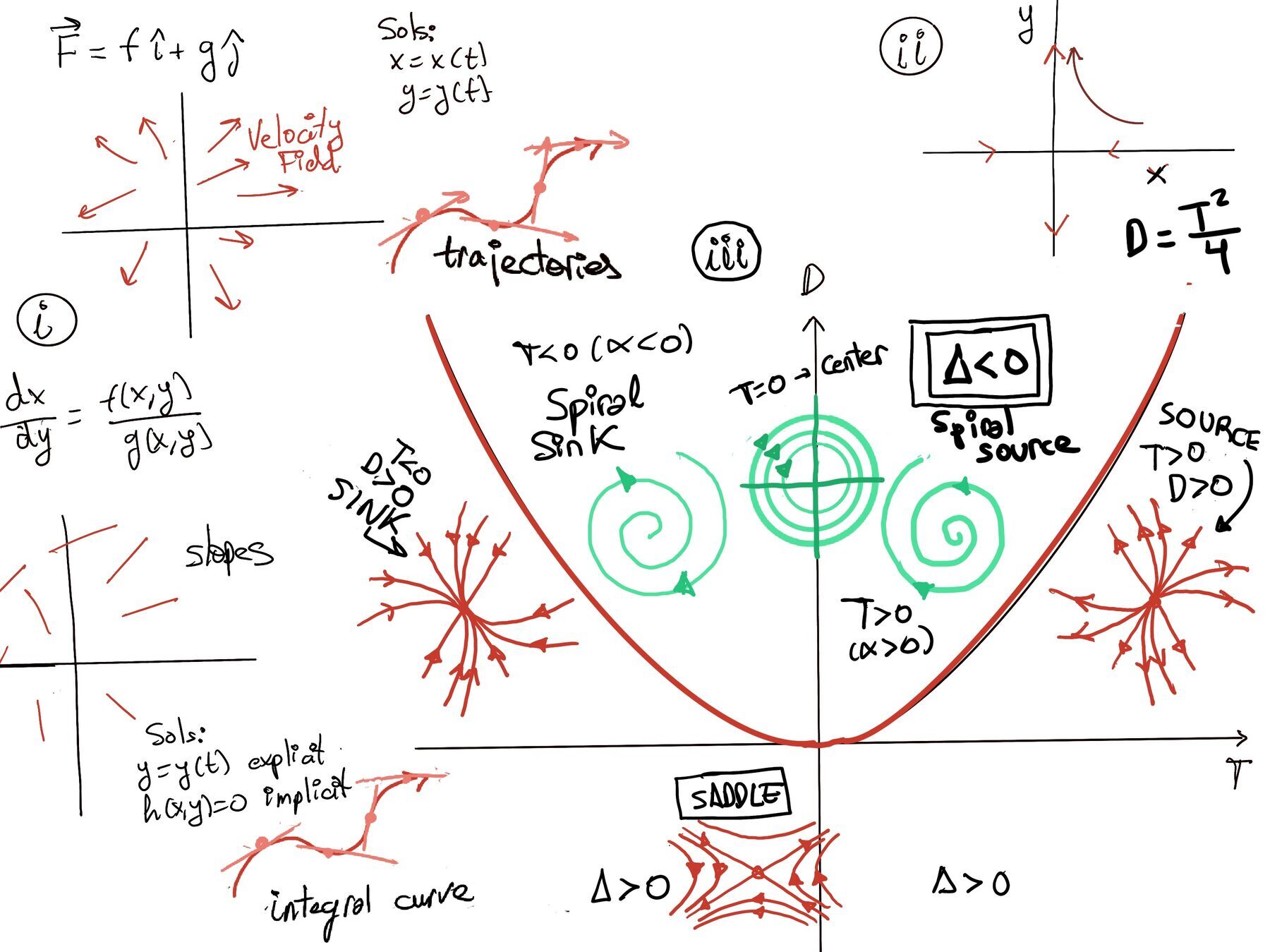
The solutions to this ODE, whether explicit y = y(x) or implicit h(x, y) = C, represent integral curves. These curves are paths in the xy-plane that have a slope matching $\frac{dy}{dx}$ at each point. By solving this ODE, we find the system’s trajectories without needing to solve for t.
Step 1: Eliminating the Parameter t
To simplify the system and analyze the trajectories in the xy-plane, we eliminate the parameter t by finding $\frac{dy}{dx}$.
$\frac{dy}{dx} = \frac{dy/dt}{dx/dt}=\frac{y'}{x'} =[\text{Substituting the expressions from equations (1) and (2):}] \frac{x + y^2}{x^2−y}$
Thus, we obtain the first-order ODE: $\frac{dy}{dx} = \frac{x + y^2}{x^2−y}$
Our next goal would normally be to solve this ODE to find the trajectories y(x). However, this specific ODE is highly non-linear and not readily solvable using standard analytical methods (it is not separable, exact, or linear). Instead, we perform a qualitative analysis to understand the system’s behavior.
Step 2: Qualitative Analysis.
Finding Critical Points Critical points occur where x’ = 0 and y’ = 0.
$\begin{cases} x^2 - y = 0 \implies y = x^2 \\ x + y^2 = 0 \end{cases}$
Substitute $y = x^2$ into the second equation: $x + (x^2)^2 = x + x^4 = 0$
Factor out x, $x(1 + x^3) = 0$
The real solutions for $x$ are $0$ and $-1$.
Therefore, the critical points are $(0, 0)$ and $(-1, 1)$.
Step 3. Linearization Around Critical Points
We can linearize the system near each critical point to analyze stability.
Compute the Jacobian matrix $J(x,y) = \begin{pmatrix} \frac{\partial f}{\partial x} & \frac{\partial f}{\partial y} \\ \frac{\partial g}{\partial x} & \frac{\partial g}{\partial y} \end{pmatrix} = \begin{pmatrix} 2x & -1 \\ 1 & 2y \end{pmatrix}$
Solving $\det(J - \lambda I) = \lambda^2 + 1 = 0 \implies \lambda = \pm i$.
The eigenvalues are purely imaginary, indicating that the linearized system predicts a center (nested closed orbits).
However, one must be careful: the Hartman-Grobman theorem fails for purely imaginary eigenvalues. Non-linear terms can push this delicate balance inward (making it a stable spiral) or outward (making it an unstable spiral). Further advanced analysis is required to confirm the true behavior at $(0,0)$.
Solving $\det(J - \lambda I) = (-2-\lambda)(2-\lambda) - (-1)(1) = \lambda^2 - 3 = 0 \implies \lambda = \pm\sqrt{3}$.
The eigenvalues are real and of opposite signs, hence the critical point $(-1, 1)$ is a saddle point. Trajectories near this point approach along a stable manifold and violently diverge along an unstable manifold.
Saddle points do not by themselves create closed orbits. Instead, they often serve as crucial boundaries (separatrices) routing traffic between different regions of trajectory behavior. This qualitative analysis allows us to understand the dynamics of the system without explicitly solving the ODE. This approach is widely used in mechanics, biology (e.g., predator-prey models), and other fields of science and engineering to analyze complex systems’ behavior.
We start with the system of differential equations that describes a simple harmonic oscillator: $\begin{cases} x' = y \\\ y' = -x \end{cases}$. Here, x and y are functions of t, and the primes denote derivatives with respect to t.
As established previously, the general solution is: $(\begin{smallmatrix}x\\\ y\end{smallmatrix}) = c_1(\begin{smallmatrix}cos(t)\\\ -sin(t)\end{smallmatrix})+c_2(\begin{smallmatrix}sin(t)\\\ cos(t)\end{smallmatrix})$ where $c_1$ and $c_2$ are constants determined by initial conditions.
Each component of the solution is a combination of sines and cosines. This is a hallmark of harmonic oscillators, whose solutions are naturally periodic functions. From the form of the solution and previous discussion, we can see that as t varies, (x(t), y(t)) traces out a circle.
This system describes a simple harmonic oscillator, and its solutions are a family of concentric circles centered at the origin (circular trajectories), representing periodic motion. Each trajectory is a closed curve, and the motion goes around clockwise indefinitely, which is typical of simple harmonic oscillators. The constant coefficients $c_1$ and $c_2$ determine the specific circle (its radius and starting point).
The motion is periodic, and each initial condition $(x_0, y_0)$ determines the circle’s radius and the starting position on that circle.
The velocity field is $\vec{F}(x,y) = y\hat{\mathbf{i}} - x\hat{\mathbf{j}}$. If we take the dot product of the position vector $\vec{r} = (x, y)$ and the velocity vector $\vec{F} = (y, -x)$, we get: $\vec{r} \cdot \vec{F} = (x)(y) + (y)(-x) = xy - xy = 0$
Because the dot product is always zero, the motion is strictly perpendicular to the radius drawn from the origin. This ensures the particle travels perfectly tangentially to a circle. The solutions are a continuous family of concentric circles centered at the origin, representing periodic motion.
Let’s arrive at the same geometric conclusion by eliminating t from the system:
$\frac{dy}{dx} = \frac{y'}{x'} = \frac{-x}{y}$. This is a separable differential equation, which can be solved as follows:
Letting $R^2 = 2C$, we get the standard implicit equation for a circle: $x^2 + y^2 = R^2$. The constant 2C corresponds to the square of the radius of each circle.
This brilliantly confirms the geometric interpretation of the original system’s solutions as circular trajectories. By eliminating time, we quickly derived the exact shape of the trajectories (concentric circles) using standard calculus, without ever needing to deal with sines, cosines, or complex eigenvalues!

JustToThePoint Copyright © 2011 - 2026 Anawim. ALL RIGHTS RESERVED. Bilingual e-books, articles, and videos to help your child and your entire family succeed, develop a healthy lifestyle, and have a lot of fun. Social Issues, Join us.
This website uses cookies to improve your navigation experience.
By continuing, you are consenting to our
use of cookies, in accordance with our Cookies Policy and
Website Terms and Conditions of use.