Basic Linear ODE. Mixing Models and Applications

The excitement of learning separates youth from old age. As long as you’re learning, you’re not old, Rosalyn S.Yalow

People are not who they say but rather who their actions reveal them to be… Be smart about it. Don’t fall for the bullshit, Ziad K. Abdelnour

Recall

Definition. A differential equation is an equation that involves one or more dependent variables, their derivatives with respect to one or more independent variables, and the independent variables themselves, e.g., $\frac{dy}{dx} = 3x +5y, y' + y = 4xcos(2x), \frac{dy}{dx} = x^2y+y, etc.$

It involves (e.g., $\frac{dy}{dx} = 3x +5y$):

• Dependent variables: Variables that depend on one or more other variables (y).
• Independent variables: Variables upon which the dependent variables depend (x).
• Derivatives: Rates at which the dependent variables change with respect to the independent variables, $\frac{dy}{dx}$

Basic linear ODE

In mathematics, a linear ordinary differential equation (ODE) is an equation involving an unknown function and its derivatives, characterized by the property that both the function and its derivatives appear linearly. This means that the unknown function and its derivatives are raised only to the first power. They are never multiplied together, nor are they composed within nonlinear functions (such as $\sin(y)$ or $e^y$). The general form for a first-order linear ODE is: a(x)y’ + b(x)y = c(x).

This property of linearity is fundamental. While most physical systems are inherently nonlinear, many can be accurately approximated by linear models over a specific range. This linearity allows mathematicians and engineers to utilize a vast and powerful toolkit of analytical solution methods that are unavailable for nonlinear systems. Consequently, linear ODEs are the bedrock of modeling in numerous fields, including:

• Fluid Dynamics: Describing fluid flow conditions under simplifications where the governing equations can be linearized.
• Electrical Circuits: Analyzing the behavior of circuits containing linear components like resistors, capacitors, and inductors (RLC circuits).
• Mechanical Vibrations: Modeling the motion of oscillating systems, such as springs and pendulums, in regimes where Hooke’s law —a linear relationship— holds.
• Radioactive Decay: Describing the constant proportional rate at which unstable atomic nuclei lose energy, resulting in exponential decay.

In this article, we will explore different forms of linear ODEs, their applications, and their solutions, with a focus on understanding their behavior in real-world contexts.

Mathematical Definition of Linearity

An ODE of order n is linear if it can be expressed in the form: $a_n(t)\frac{d^ny}{dt^n} +a_{n-1}(t)\frac{d^{n-1}y}{dt^{n-1}} + ··· + a_1(t)\frac{dy}{dt} + a_0(t)y = q(t)$ where

• y(t) is the unknown function (dependent variable).
• i is the independent variable.
• $\frac{d^ky}{dt^k}$ are the derivatives of y with respect to t.
• a_i(t) are known coefficient functions of t. They can be constants or functions of t, but they do not depend on y.
• q(t) is a known function, often called the forcing function or input.

The function y and its derivatives appear to the first power and are not multiplied together.

Homogeneous vs. Non-Homogeneous Equations

A crucial classification for linear ODEs depends on the forcing function $q(t)$.

1. Homogeneous Linear ODE: If the forcing function is identically zero ($q(t) = 0$), the equation is said to be homogeneous:
   $a_1(t)y' + a_0(t)y = 0$.
   The trivial solution, $y(t)=0$, always satisfies a homogeneous equation.

2. Non-Homogeneous Linear ODE: If the forcing function is not zero ($q(t) \neq 0$), the equation is non-homogeneous:
   $a_1(t)y' + a_0(t)y = q(t)$
   The general solution to a non-homogeneous equation is composed of the sum of the general solution to its associated homogeneous equation and a particular solution to the non-homogeneous equation.

Common Forms of First-Order Linear ODEs

First-order linear ODEs involve only the unknown function and its first derivative. Mastering these forms is the foundational step toward understanding more complex higher-order systems. They commonly appear in several equivalent structures:

• Standard Linear Form. This is the most mathematically general structure, widely used in textbook solution methods (such as integrating factors): y’ + p(t)y = q(t), where y is the unknown function of time, p(t) is a function of time, and q(t) is a known function representing external input or forcing. Examples: $\frac{dy}{dt} + sin(t)y = e^t$ where p(t) = sin(t) and $q(t) = e^t.

• Constant Coefficient Form. A specific and very common case where the coefficient of y is a positive constant (k > 0) and q(t) represent an external (forcing) input. This structure often describes systems with natural decay or resistance: y’ + ky = q(t). Example: $\frac{dy}{dt}+ 3y = \cos(t)$ where k = 3 and q(t) = cos(t).

• Proportional Input Form. This form is widely used in systems engineering and physical modeling. It expresses the forcing function ($kq_e(t)$ in terms of the system’s “speed” constant, k:) y’ + ky = kq_e(t), where $kq_e(t)$ represents the dimensionless external input, and k dictates how strongly the system couples to that input. Examples: $\frac{dy}{dt}+2y=2e^{2t}$ where k = 2 and q_e(t) = e^2t.

Each of these forms arises in different real-world scenarios, which we will break down further.

Physical Application: Salt Mixing in a Tank

Deriving mathematical models for mixing substances is a prerequisite in chemical engineering, pharmacology, and environmental science.

Consider a well-mixed tank containing a solution of salt and water. A saltwater mixture flows in, and the well-mixed solution flows out. Let’s model how the mass of salt in the tank changes over time.

Let’s define the variables involved:

• V is the volume of the solution in the tank. The volume V of the solution (constant, L or gal) in the tank remains constant because the inflow and outflow rates are equal.

• r represents the flow rate (volume per unit time, e.g., liters or gallons per minute or hour). The rate at which the solution flows into and out of the tank is constant.

• x(t) is the total amount of salt in the tank at time t (mass, e.g., kilograms or grams).

• C_e(t) is the concentration of incoming salt as a function of time (mass per unit volume, e.g., kg/L, refer to Figure E for a visual representation and aid in understanding it).

• C(t): Concentration of salt in the tank at time t (mass per unit volume).

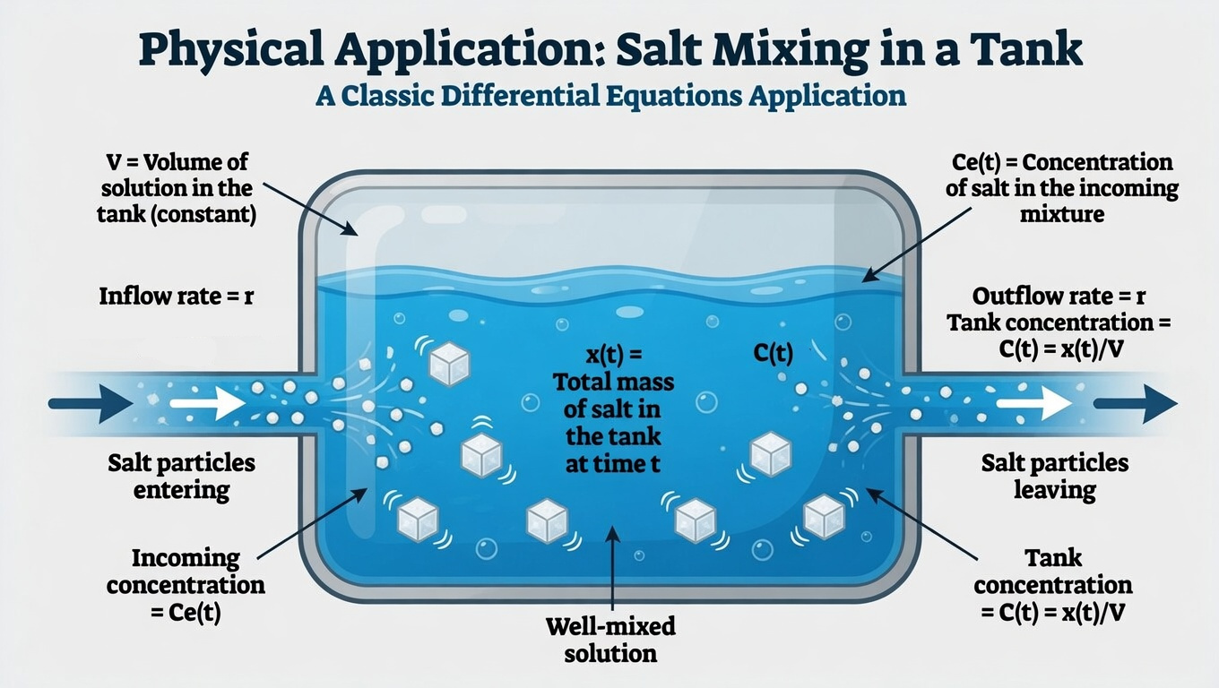
The tank is well-mixed, so the concentration of salt throughout the tank is uniform at all times, meaning the concentration of salt is uniform throughout the tank. Therefore, $C(t) = \frac{x(t)}{V}$

Deriving the ODE via Conservation of Mass

The fundamental modeling principle is the principle of conservation of mass: the rate of change of the amount of substance in the tank equals the rate at which it enters minus the rate at which it leaves.

Mathematically, this translates to the differential equation:

$\frac{dx}{dt} = \text{Rate of Salt Inflow − Rate of Salt Outflow}$

Where the rates of salt flow are calculated as (Flow Rate) × (Concentration): $\text{Rate}_{\text{in}} = r \cdot C_e(t)$; $\text{Rate}_{\text{out}} = r \cdot C(t) = r \cdot \frac{x(t)}{V}$

Substituting these definitions into the conservation principle yields: $\frac{dx}{dt} = rC_e(t) - r\frac{x}{V}$

Rearranging terms to the standard form gives: $\boxed{\frac{dx}{dt} + \left(\frac{r}{V}\right)x = rC_e(t)}$

This equation states that the rate of change of salt in the tank $\frac{dx}{dt}$ is equal to the rate of salt inflow (the product of the inflow rate r and the concentration of the incoming solution C_e(t)) r·C_e(t) minus the rate of salt outflow (the product of the outflow rate r and the concentration of the solution in the tank C(t):) $r·\frac{x}{V}$, where C(t) = ^x⁄_V is the concentration of salt in the tank at time t (since the tank is well-mixed).

Expressing the Equation in Terms of Concentration

While the above equation describes the total mass x(t), scientists often find concentration C(t) to be a more practical variable. Recalling that C(t) = ^x⁄_V, x(t) = VC(t) we differentiate with respect to time: $\frac{dx}{dt} = \frac{d}{dt}(VC(t)) =[\text{V is constant}] V \frac{dC}{dt}$, and we get: $V \frac{dC}{dt} + rC = rC_e(t)$

Dividing the entire equation by the constant volume V: $\frac{dC}{dt} + (\frac{r}{V})C = (\frac{r}{V})C_e(t)$.

Physical Significance of the Parameter k

Let’s define a new parameter, $k = r/V$. This is known as the dilution rate or the fractional flow rate, and its unit is inverse time ($1/t$, e.g., $1/\text{min}$). Physically, $k$ represents the fraction of the total tank volume that is replaced per unit time. It dictates the “speed” of the system

Substituting $k$ back into the concentration equation yields the generic dynamic model: $\boxed{\frac{dC}{dt} + kC = kC_e(t)}$

This is a first-order linear ordinary differential equation in proportional input form describing the salt concentration in the tank.

Intuitive Understanding of the Model

• Large k: the flow rate is high or the volume is small, so the concentration of salt in the tank C(t) rapidly matches or adjusts to the incoming concentration C_e(t). The system responds swiftly to changes in C_e(t).
• Small k: the flow rate is low or the volume is large, the system has a delayed response to changes in C_e(t). It takes longer for the concentration in the tank C(t) to catch up with the incoming concentration C_e(t).
• If C_e(t) changes over time, e.g., it is a sinusoidal function (e.g., C_e(t) = cos(wt)), the concentration C(t) will also oscillate but may lag behind (with a phase lag Φ) and reduced amplitude depending on k.

Solving the Dynamic Mixing Model

The generic first-order linear ODE derived above can be solved explicitly using the integrating factor method, $\frac{dC}{dt} + kC = kC_e(t)$

1. Compute the Integrating Factor μ(t): $μ(t) = e^{\int kdt} = e^{kt}$
2. Multiply both sides of the ODE by μ(t): $e^{kt}\frac{dC}{dt} + ke^{kt}C = ke^{kt}C_e(t)$. The left-hand side of the equation simplifies to: $\frac{d}{dt}(e^{kt}C)$
3. Integrate Both Sides: $\int \frac{d}{dt}(e^{kt}C)dt = \int ke^{kt}C_e(t)dt ↭ e^{kt}C = k\int e^{kt}C_e(t)dt + C_1$ where C₁ is the constant of integration determined by the initial concentration C(0).
4. Solve for the Concentration C(t): $\boxed{C(t) = e^{-kt}[k\int e^{kt}C_e(t)dt + C_1]}$

This explicit solution allows engineers to predict the tank concentration C(t) over time for any initial condition C(0) and any varying incoming concentration profile $C_e(t)$.

Special Case: Constant Input Concentration

Consider the dynamic mixing mode $\frac{dC}{dt} + kC = kC_e(t)$, where k is the system rate constant (defined as flow rate r / tank volume V).

Suppose the concentration of the incoming substance, $C_e(t)$ is not changing over time. We define this constant input as $C_{input}$ or $C_0$.

1. Integrate the Right-Hand side: $\int e^{kt}C_e(t)dt = C_0\int e^{kt}dt = \frac{C_0e^{kt}}{k} + C_2$
2. Substitute back into the solution: $C(t) = e^{-kt}[k\int e^{kt}C_e(t)dt + C_1] = e^{-kt}[k(\frac{C_0e^{kt}}{k}) + kC_2 + C_1] = C_0 + kC_2e^{-kt} + C_1e^{-kt} = C_0 + (kC_2+C_1)e^{-kt} = C_0 + C'e^{-kt}$. $\boxed{C(t) = C_0 + C'e^{-kt}}$ where $C' = kC_2+C_1$. This is the general solution for concentration under constant input.
   The term $C_0$ represents the long-term stable concentration, and $C'e^{-kt}$ represents the system’s adjustment from its starting point.
3. Applying Initial Conditions. Suppose we have an initial condition C(0) = C_initial: $C_{initial} = C_0 + C'e^{-0·t} = C_0 + C'⇒ C' = C_{initial} -C_0$. The general solution to the differential equation with a constant input concentration is: $C(t) = C_0 + (C_{initial} -C_0)e^{-kt}$

This expression is a highly effective “shortcut formula” that models how any first-order constant input system moves from its initial state ($C_{initial}$) to its new input driving state ($C_{input}=C_0$).

Interpretation

Breaking down this solution formula into its parts gives us complete operational insight into the system dynamics over time:

• Steady-State Solution (The Destination): As t → ∞, the exponential term $e^{-kt}$ decays exponentially to zero, the entire term $(C_{initial} -C_0)e^{-kt}$ vanishes, so C(t) → C₀. This means that no matter what the tank's initial concentration was, the concentration in the tank will eventually perfectly match the driving input concentration $C_0 = C_{input}$.
• Transient Solution (The Journey): The term $(C_{initial} -C_0)e^{-kt}$ represents the temporary or transient behavior. It captures the adjustment phase where the system is leaving its old state $C_{initial}$ and moving toward the new state $C_0 = C_{input}$. This behavior is temporary and decays over time.
• Rate of Convergence (The Speedometer): The magnitude of the system constant k (which is r/V) dictates how fast the transient term decays. A large k (high flow rate relative to tank volume) creates a very rapid decay, meaning the system snaps quickly from initial state to input state. A small k (low flow relative to volume) results in a slow decay, meaning the system takes a long time to converge to the input state.

Improved Example Problem Solution

By applying the specific solution formula for constant input derived above, we can solve complex physical problems, like the beer vat mixing scenario, much more efficiently and with fewer constant variables than using re-integration from scratch.

A vat contains 500 gallons of beer with an alcohol concentration of 4% (by volume). Beer with an alcohol concentration of 7% is pumped into the vat at a rate of 5 gallons per minute. The mixture is simultaneously pumped out at the same rate. Questions: (a) What is the amount of alcohol in the vat after an hour? (b) What is the percentage of alcohol after an hour?

Step 1: Define Physical Variables and System Constants: The vat contains V = 500 gallons of beer with C_initial = 4% = 0.04 alcohol, so initially, the amount of alcohol is: A(0) = V·C_initial = 500 × 0.04 = 20 gallons of alcohol. Inflow and Outflow Rate: r = 5 gal/min. Incoming Alcohol Concentration: C_e(t) = 7% = 0.07.

Step 2: Set Up the Differential Equation

Let A(t) be the amount of alcohol in the vat at time t (measured in gallons). The concentration of alcohol in the vat at time t is: $C(t) = \frac{A(t)}{V} = \frac{A(t)}{500}$ because concentration = ^{amount of alcohol}⁄_volume.

The rate of alcohol inflow and outflow can be written as: $\frac{dA}{dt} = \text{Rate of Alcohol Inflow - Rate of Alcohol Outflow} = rC_e(t) -r\frac{A(t)}{V} = 5\text{gal/min}·0.07 -5\text{gal/min}·\frac{A}{500}$

• Rate of inflow: Beer with 7% alcohol is being pumped in at 5 gal/min, so the rate of alcohol inflow is: 5 gal/min × 0.07 = 0.35 gal/min.
• Rate of outflow: The mixture is being pumped out at the same rate of 5 gal/min, and the concentration of alcohol in the vat at any time t is ^A(t)⁄₅₀₀ where A(t) is the amount of alcohol at time t. Thus, the rate of alcohol outflow is: 5 gal/min x ^A(t)⁄₅₀₀ = 0.01·A(t).

Thus, the differential equation becomes: $\frac{dA}{dt}=0.35 -0.01A, A(0) = 20, A(60)?$

Step 3: Solve the Differential Equation. This is a separable differential equation. Let’s separate the variables: $\frac{1}{0.35 -0.01A}dA = dt$.

Integrate both sides: $\int \frac{1}{0.35 -0.01A}dA = \int dt ⇒ \frac{1}{-0.01}ln|0.35 -0.01A| = t + C_1 ⇒[\text{Simplifying:}] ln|0.35 -0.01A| = -0.01(t + C_1) ↭ ln|0.35 -0.01A| = -0.01t + C_2$ where C₂ = -0.01·C₁ is a new constant of integration.

On the left-hand side, the integral requires a substitution u = 0.35 - 0.01A, so du = -0.01dA.

$ln|0.35 -0.01A| = -0.01t + C_2 ↭[\text{Take exponentials of both sides to solve for A:}] |0.35 -0.01A| = e^{-0.01t + C_2}↭ |0.35 -0.01A| = C_3e^{-0.01t}$ where C₃ = e^C₂

$0.35 -0.01A = ± C_3e^{-0.01t} ↭ -0.01A = -0.35 + C_4e^{-0.01t}$ where C₄ = ± C₃.

Solving for A, $A = \frac{-0.35}{-0.01}+\frac{C_4}{-0.01}e^{-0.01t} ↭ A = 35 + C_5e^{-0.01t}$ where $C_5 = \frac{C_4}{-0.01}⇒[\text{Let C = C₅. Applying the initial conditions}] A(0) = 20 = 35 + Ce^{-0.01·0} ↭ C = 20 -35 = -15 ⇒[\text{Thus, the general solution is:}] A = 35 + Ce^{-0.01t} = 35 -15e^{-0.01t}$

Step 4: Calculate Amount of Alcohol After One Hour (60 minutes). $A(60) = 35 -15e^{-0.01·60} = 35 -15e^{-0.6}≈ 26.77$ gallons of alcohol. So, after an hour (60 minutes), the vat contains approximately 26.7 gallons of alcohol.

Step 5: Calculate the Percentage of Alcohol After One Hour. Alcohol Concentration = $\frac{A(60)}{500} x 100$% $= \frac{26.77}{500} x 100 = 0.0535 x 100 = 5.35$% is the percentage of alcohol after an hour. After 60 minutes, the alcohol concentration has risen from its initial 4% up to approximately 5.35%, trending toward the input of 7%.

Bibliography

1. NPTEL-NOC IITM, Introduction to Galois Theory.
2. Algebra, Second Edition, by Michael Artin.
3. LibreTexts, Calculus and Calculus 3e (Apex). Abstract and Geometric Algebra, Abstract Algebra: Theory and Applications (Judson).
4. Field and Galois Theory, by Patrick Morandi. Springer.
5. Michael Penn, and MathMajor.
6. Contemporary Abstract Algebra, Joseph, A. Gallian.
7. YouTube’s Andrew Misseldine: Calculus. College Algebra and Abstract Algebra.
8. MIT OpenCourseWare [18.03 Differential Equations, Spring 2006], YouTube by MIT OpenCourseWare.
9. Calculus Early Transcendentals: Differential & Multi-Variable Calculus for Social Sciences.