Basic linear ODE. Electrical Circuits (RC Circuit).

You have enemies? Good. That means you’ve stood up for something, sometime in your life, Winston Churchill

Recall

Definition. A differential equation is an equation that involves one or more dependent variables, their derivatives with respect to one or more independent variables, and the independent variables themselves, e.g., $\frac{dy}{dx} = 3x +5y, y' + y = 4xcos(2x), \frac{dy}{dx} = x^2y+y, etc.$

It involves (e.g., $\frac{dy}{dx} = 3x +5y$):

• Dependent variables: Variables that depend on one or more other variables (y).
• Independent variables: Variables upon which the dependent variables depend (x).
• Derivatives: Rates at which the dependent variables change with respect to the independent variables, $\frac{dy}{dx}$

Basic linear ODE

In mathematics, a linear ordinary differential equation (ODE) is an equation involving an unknown function and its derivatives, characterized by the property that both the function and its derivatives appear linearly. This means that the unknown function and its derivatives are raised only to the first power. They are never multiplied together, nor are they composed within nonlinear functions (such as $\sin(y)$ or $e^y$). The general form for a first-order linear ODE is: a(x)y’ + b(x)y = c(x).

This property of linearity is fundamental. While most physical systems are inherently nonlinear, many can be accurately approximated by linear models over a specific range. This linearity allows mathematicians and engineers to utilize a vast and powerful toolkit of analytical solution methods that are unavailable for nonlinear systems. Consequently, linear ODEs are the bedrock of modeling in numerous fields, including:

• Fluid Dynamics: Describing fluid flow conditions under simplifications where the governing equations can be linearized.
• Electrical Circuits: Analyzing the behavior of circuits containing linear components like resistors, capacitors, and inductors (RLC circuits).
• Mechanical Vibrations: Modeling the motion of oscillating systems, such as springs and pendulums, in regimes where Hooke’s law —a linear relationship— holds.
• Radioactive Decay: Describing the constant proportional rate at which unstable atomic nuclei lose energy, resulting in exponential decay.

In this article, we will explore different forms of linear ODEs, their applications, and their solutions, with a focus on understanding their behavior in real-world contexts.

Mathematical Definition of Linearity

An ODE of order n is linear if it can be expressed in the form: $a_n(t)\frac{d^ny}{dt^n} +a_{n-1}(t)\frac{d^{n-1}y}{dt^{n-1}} + ··· + a_1(t)\frac{dy}{dt} + a_0(t)y = q(t)$ where

• y(t) is the unknown function (dependent variable).
• i is the independent variable.
• $\frac{d^ky}{dt^k}$ are the derivatives of y with respect to t.
• a_i(t) are known coefficient functions of t. They can be constants or functions of t, but they do not depend on y.
• q(t) is a known function, often called the forcing function or input.

The function y and its derivatives appear to the first power and are not multiplied together.

In this second article, we will continue exploring different forms of linear ODEs, their applications, and their solutions, with a focus on understanding their behavior in real-world contexts.

Electrical Circuit (RC Circuit)

An RC circuit is a fundamental electrical circuit combining a resistor (R) and a capacitor (C) connected in series or parallel with a voltage source. Understanding the behavior of an RC circuit is crucial in fields like electrical engineering and physics because it illustrates how circuits respond over time to changes in voltage. This response is characterized by the charging and discharging of the capacitor, which is governed by a first-order linear ordinary differential equation (ODE).

Components of the RC Circuit

• A resistor (R) opposes the flow of electric current, converting electrical energy into heat. It is measured in ohms (Ω). Its primary function is to resist current, effectively controlling how fast the capacitor charges or discharges by limiting the magnitude of that current.
• A capacitor (C) stores electrical energy in an electric field established between its internal plates. It is measured in farads (F). It accumulates electric charge dynamically, released later to provide power or smooth out voltage variations. Capacitance defines this charge-storage ability.
• A Voltage Source (ε(t)) acts as the driving force, providing electrical energy to the circuit. It can deliver constant voltage (like a battery) or vary with time (like AC supplies), propelling the current that dynamically charges or discharges the capacitor.

Governing Differential Equation

In an RC circuit, the relationship between the charge q(t) on the capacitor, the current i(t), and the applied voltage ε(t) is governed by the following first-order linear ordinary differential equation (ODE): $R\frac{dq}{dt}+\frac{q(t)}{C}=ε(t)$ where:

• q(t) represents the electric charge stored in the capacitor at time t (in columbus, C).
• $\frac{dq}{dt}$ is the rate of change of charge with respect to time. This is equivalent to the current i(t) flowing through the circuit, defined as $i(t) = \frac{dq}{dt}$.
• R is the resistance. This component resists the flow of electric current, measured in ohms (Ω).
• C is the capacitance. This defines the ability of a capacitor to store charge, measured in farads (F). A capacitor is like a tiny rechargeable battery that stores electrical energy in an electric field. Later, this stored charge can be released to do work, like powering a circuit or smoothing out voltage fluctuations.
• ε(t) is the voltage supplied by the voltage source, which can be constant or time-dependent (Refer to Figure F for a visual representation and aid in understanding it).

Derivation of the Differential Equation

This equation is derived by applying cornerstone circuit laws:

1. Ohm’s Law: The relationship between voltage (V), current (i), and resistance (R) is defined by Ohm’s Law. The voltage across the resistor is directly proportional to the current: $V_R = i(t)R =[\text{Since current is the rate of change of charge, } i(t) = \frac{dq}{dt}]$, we can write $V_R = R \cdot \frac{dq}{dt}$
2. Capacitor Voltage: The voltage across the capacitor is proportional to the stored charge: $V_C = \frac{q(t)}{C}$.
3. Kirchhoff’s Voltage Law (KVL): The sum of the voltage drops around any closed loop must equal the supplied voltage. So, the voltage drop across the resistor ($V_R$) plus the voltage drop across the capacitor ($V_C$) equals the source voltage: $V_R + V_C = ε(t)$

$V_R + V_C = ε(t)$ ↭[Substitute V_R (Ohm’s Law) and V_C (Voltage Across Capacitor):] $\boxed{R·\frac{dq}{dt} + \frac{q(t)}{C} = ε(t)}$

This is a first-order linear ordinary differential equation, describing the dynamically evolving charge q(t). The time-varying current is implicitly captured by $\frac{dq}{dt}$, meaning the circuit’s overall response is characterized by the charging and discharging of the capacitor.

Standard Form of the Differential Equation

To solve the differential equation, we rewrite it in standard linear form: $\frac{dq}{dt}+\frac{1}{RC}q = \frac{ε(t)}{R}$.

Using the notation q’ = $\frac{dq}{dt},\text{ we have } q' +\frac{1}{RC}q = \frac{ε(t)}{R}$

This equation is a first-order linear ordinary differential equation, which can be solved using an integrating factor.

Solving the Differential Equation

1. Identify P(t) and Q(t). The standard form of a first-order linear ODE is: y′+P(t)y = Q(t). For our equation: y = q, P(t) = ¹⁄_RC (a constant), Q(t) = ^ε(t)⁄_R.
2. Calculate the Integrating Factor μ(t): $μ(t) = e^{\int P(t)dt} = e^{\int \frac{1}{RC}dt} = e^{\frac{t}{RC}}$
3. Multiply Both Sides by μ(t): $e^{\frac{t}{RC}}q' +e^{\frac{t}{RC}}(\frac{1}{RC}q) = e^{\frac{t}{RC}}·\frac{ε(t)}{R}$. Simplify the left side using the product rule: $\frac{d}{dt}(e^{\frac{t}{RC}}·q) = e^{\frac{t}{RC}}·\frac{ε(t)}{R}$
4. Integrate Both Sides: $e^{\frac{t}{RC}}·q = \int e^{\frac{t}{RC}}·\frac{ε(t)}{R}dt + C'$ where C’ is the constant of integration.
5. Solve for $\boxed{q(t) = e^{\frac{-t}{RC}}(\int e^{\frac{t}{RC}}·\frac{ε(t)}{R}dt + C')}$

Analyzing the Solution

The general solution q(t) consists of two components:

1. Homogeneous Solution (Natural Response): $q_h(t) = C'e^{\frac{-t}{RC}}$.
   This term represents the natural response or transient behavior, dictating how any initial charge decays exponentially to zero if the external source is removed.
2. Particular Solution (Forced Response): $q_p(t) = e^{\frac{-t}{RC}}\int e^{\frac{t}{RC}}·\frac{ε(t)}{R}dt$. Depends on the specific form of the forcing voltage ε(t) and signifies the steady-state response, illustrating how the circuit responds over time to the voltage source.

Example: Constant Voltage Source ε(t) = E

For a constant voltage source, the specific solution, incorporating the natural and forced responses, is explicitly derived:

1. Integrate the right side: $\int e^{\frac{t}{RC}}\cdot \frac{ε(t)}{R}dt = \int e^{\frac{t}{RC}}\cdot \frac{E}{R}dt = \frac{E}{R}\int e^{\frac{t}{RC}} dt = \frac{E}{R}·RC·e^{\frac{t}{RC}} = EC·e^{\frac{t}{RC}}$.
2. Plug back into the solution: $q(t) = e^{\frac{-t}{RC}}(EC·e^{\frac{t}{RC}} + C') = EC + C'e^{\frac{-t}{RC}}$
3. Determine the Constant C’ Using Initial Conditions q(0) = q₀. q₀ = EC + C’ ⇒ C’ = q₀ - EC.
   The specific solution, incorporating the natural and forced responses, is: $\boxed{q(t) = EC + (q_0 -EC)e^{\frac{-t}{RC}}}$ where $q_0$ is the initial charge on the capacitor at time t = 0, determined by the initial condition.

The resulting dynamic current i(t) is simply the derivative: i(t) = $\frac{dq}{dt} = \frac{d}{dt}(EC) + \frac{d}{dt}((q_0 -EC)e^{\frac{-t}{RC}}) = 0 +(q_0 -EC)\frac{-1}{RC}e^{\frac{-t}{RC}} = -\frac{q_0 -EC}{RC}e^{\frac{-t}{RC}}$.

Interpretation

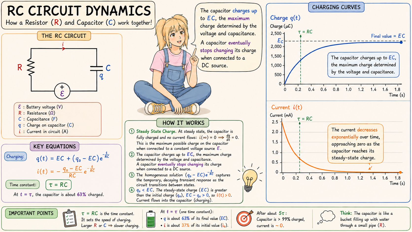
• Steady State Charge, $q_{SS} = EC$.
  At steady state, the capacitor is fully charged and no current flows: $i(\infty) = 0 \implies \frac{dq}{dt} = 0$.
  Plug this into the ODE: $R \cdot 0 + \frac{q_{\infty}}{C} = E \implies q_{\infty} = EC$. This is the maximum possible charge on the capacitor when connected to a constant voltage source 𝐸.
  🧩 It depends only on the voltage and the capacitance. It does not depend on the resistance 𝑅. Resistance only controls how fast you get there.
  As time progresses indefinitely ($t \to \infty$), the exponential term $e^{-\frac{t}{RC}}$ approaches zero. The homogeneous natural response decays completely. The capacitor dynamically approaches a steady-state charge, The capacitor charges up to EC, the maximum charge determined by the voltage and capacitance. $q(t) \to EC, i(t) \to 0$. A capacitor eventually stops changing its charge when connected to a DC source. No change in charge → no current.

• Transient Behavior: The homogeneous solution $(q_0 -EC)e^{\frac{-t}{RC}}$ captures the temporary, decaying transient response as the circuit transitions between states. The direction and magnitude of the current change are indicates how much of a current will flow into or out of the capacitor dynamically:

  ($\star$) Charging. $q_0 \lt EC$. The steady-state charge (EC) is greater than the initial charge ($q_0$), $EC - q_0 \gt 0$, so i(t) > 0. Current flows into the capacitor (charging), increasing its charge towards EC. The current decreases exponentially over time, approaching zero as the capacitor reaches its steady-state charge.
  ($\star$) Discharging. $q_0 \gt EC$. The steady-state charge is smaller than the initial charge, $EC - q_0 \lt 0$, so i(t) < 0. Current flows out of the capacitor, reducing its stored charge towards EC. In both cases, the exponential term shrinks, so the current decays to zero.

• The time constant τ is a key parameter: τ = RC. It determines the rate at which the capacitor charges or discharges.

The larger the resistance or capacitance, the longer it takes for charge to build or decay. After one time constant (t = τ), the transient term decays to approximately $e^{\frac{-t}{RC}} = e^{-1} ≈0.3679$, meaning the process is roughly 1 - 0.37 = 63% complete.

In other words, the capacitor has completed 63% of the journey toward steady state.

The Hydraulic Metaphor Breakdown

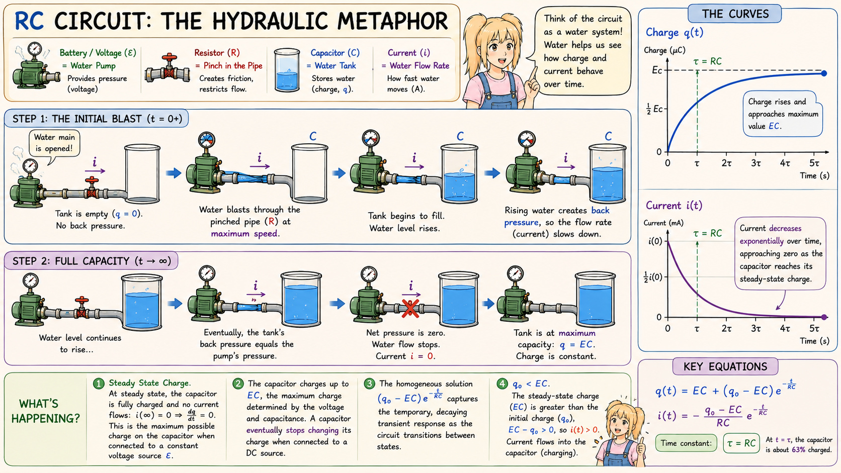
The most powerful way to visualize this is as a filling tank broken down into chronological steps.

• The Battery / Voltage (ε) is the Water Pump: It provides the “pressure” (voltage) pushing the water (electrons) through the system.

• The Resistor (R) is a Pinch in the Pipe: A narrow section of pipe creates friction, restricting how much water can flow through at once. A higher resistance means a narrower pipe.

• The Capacitor (C) is a Water Tank: As water flows in, the tank fills up (storing charge, q).

• Current (i) is the Water Flow Rate: It is how fast the water is moving through the pipes at any given second.

The cartoon infographic helps you map these specific behaviors to the components:

Step 1: The Initial Blast: The water main is opened. The storage tank is empty, so there is zero back pressure. Water blasts through the pinched pipe (the resistor) at maximum speed. This is the high-flow point on the Current graph.

Filling Chronology (The curves): As water flows in, the water level in the tank rises (Charge curves up). But as it rises, that water creates its own pressure, pushing back against the pump. Since the net pressure in the system is dropping, the current flow must slow down (Current curves down).

Step 2: Full Capacity: Eventually, the tank’s back pressure exactly matches the pump’s forward pressure. The net pressure is zero. The water flow stops entirely (Current is zero), and the tank is sitting at its maximum capacity (Charge is flat/constant).

Bibliography

1. NPTEL-NOC IITM, Introduction to Galois Theory.
2. Algebra, Second Edition, by Michael Artin.
3. LibreTexts, Calculus and Calculus 3e (Apex). Abstract and Geometric Algebra, Abstract Algebra: Theory and Applications (Judson).
4. Field and Galois Theory, by Patrick Morandi. Springer.
5. Michael Penn, and MathMajor.
6. Contemporary Abstract Algebra, Joseph, A. Gallian.
7. YouTube’s Andrew Misseldine: Calculus. College Algebra and Abstract Algebra.
8. MIT OpenCourseWare [18.03 Differential Equations, Spring 2006], YouTube by MIT OpenCourseWare.
9. Calculus Early Transcendentals: Differential & Multi-Variable Calculus for Social Sciences.