Now is the time for us to shine. The time when our dreams are within reach and possibilities vast. Now is the time for all of us to become the people we have always dreamed of being. This is your world. You’re here. You matter. The world is waiting, Haley James Scott.

image info

Recall

Definition. A function f is a rule, relationship, or correspondence that assigns to each element x in a set D, x ∈ D (called the domain) exactly one element y in a set E, y ∈ E (called the codomain or range).

The pair (x, y) is denoted as y = f(x) where: x is the independent variable (input) and y is the dependent variable (output). Often, both the domain D and codomain E are the set of real numbers ℝ or subsets of ℝ.
D is the domain, the set of all possible inputs. E is the codomain or range, the set of all possible outputs.
Key property💡: Each input has exactly one output. (No input is assigned two different outputs — this is the vertical line test!)
Examples: constant, f(x) = c, horizontal line, slope = 0; linear, f(x) = mx + b, straight line, constant slope m and y-intercept b; quadratic $f(x) = ax^2 + bx + c$, u-shaped or inverted U, opens up (a > 0) or down (a < 0), vertex at x = $\frac{-b}{2a}$, symmetry about vertical axis through vertex; polynomial, $f(x) = a_n x^n + \dots + a_0$, a smooth and continuous curve, n roots (counting multiplicity), end behaviour determined by its leading term $a_n x^n$; exponential function, $f(x) = a \cdot b^x, a \ne 0, b \gt 0$, rapid growth (b > 1) or decay (0 < b < 1); trigonometric functions, $\sin(x), \cos(x), \tan (z)$ oscillatory, periodic behavior (period 2π for sin/cos, π for tan), sin and cos are bounded between -1 and 1, but tan is unbounded; step function $f(x) = \lfloor x \rfloor$, greatest integer ≤ x, constant on intervals [n, n+1), jumps at integers, its graph is a staircase shape; absolute value f(x) = |x|, V-shaped graph, slope changes at 0.
Functions can be expressed in multiple forms, each useful in different contexts: verbal description, table of values (list of pairs), algebraic formula, graph, piecewise definition, recursive definition, parametric or integral form, and series representation.
Evaluating a function means finding or computing the output value f(x) for a given input value x. f(x) = $x^2-2x +4, f(2) = 2^2 -2\cdot 2 + 4 = 4 - 4 + 4 = 4, f(0) = 0^2 -2\cdot 0 + 4 = 4, f(1) = 1^2 -2\cdot 1 + 4 = 1 -2 +4 = 3$
The x-intercept is any point on the graph that intersects or crosses the x-axis. In other words, it is the value of x when the function (y-coordinate or y-value) is zero. The y-intercept is the point where the graph intersects or crosses the y-axis. y-coordinate of the point whose x-coordinate is 0, e.g., 2x - 3y = 6. x-intercept: set y = 0 → 2x = 6 ⇒ x=3, so (3, 0). y-intercept: set x = 0 → −3y = 6 ⇒ y = −2, so (0, −2).
f is said to have a local or relative maximum at c if there exists an interval (a, b) containing c ($c \in (a, b)$) such that f(c) ≥ f(x) $∀ x \in (a, b) ∩ D$. f is said to have a local or relative minimum at c if there exists an interval (a, b) containing c ($c \in (a, b)$) such that f(c) ≤ f(x) $∀ x \in (a, b) ∩ D$.💡Local extrema can only occur where the function stops rising or falling —either because the derivative is zero, the derivative doesn't exist, or you're at the edge of the domain.
First Derivative Test. Let f be differentiable on an open interval containing c, except possibly at c itself, and let c be a critical point (so f′(c) = 0 or f′ is undefined). Then:

If f′(x) > 0 for x just to the left of c and f′(x) < 0 for x just to the right of c, then f(c) is a local maximum.
If f′(x) < 0 for x just to the left of c and f′(x) > 0 for x just to the right of c, then f(c) is a local minimum.
If f′(x) does not change sign at c (stays positive or stays negative), then f(c) is not a local extremum.

Second Derivative Test. If the first derivate of a function at a point c is zero (f'(c) = 0) and the second derivate at this point exists, then: (i) If f''(c) > 0, then f(c) is a local minimum. (ii) If f''(c) < 0, then f(c) is a local maximum. (iii) If f''(c) = 0, the test is inconclusive.

Asymptotes and End Behavior of Functions

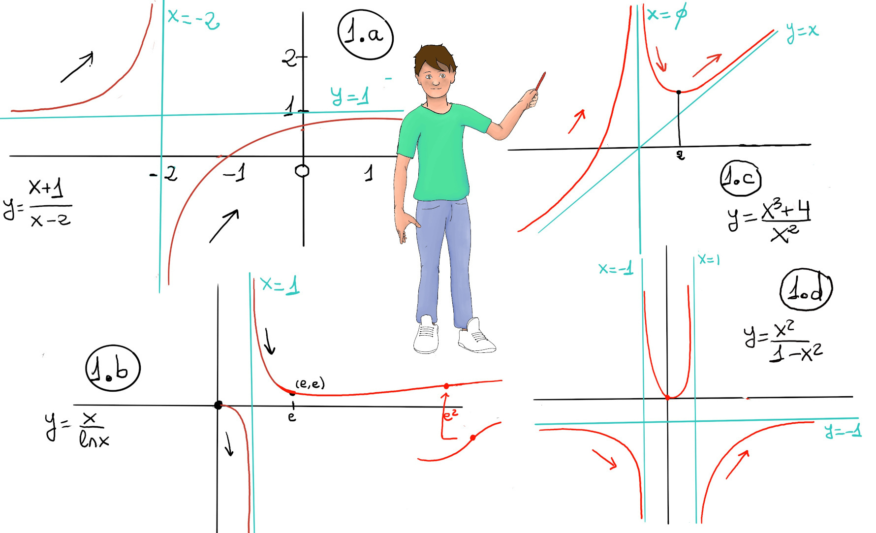
An asymptote is an horizontal, vertical, or slanted line such that the distance between the graph and the line approaches zero as the independent variable tends to infinity (or to a finite singular point). In other words, it is a line L that the graph approaches (it gets closer and closer, but never quite reach) as it heads or goes to positive or negative infinity or to some finite x-value.

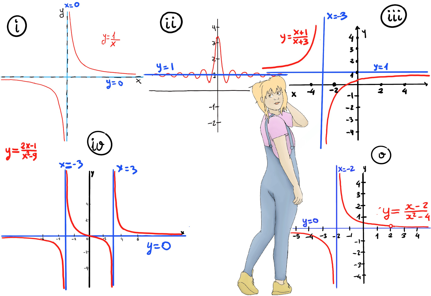
Vertical asymptotes are vertical lines (perpendicular to the x-axis) of the form x = a (where a is a constant) near which the function grows without bound when x approaches a from at least one side. The line x = a is a vertical asymptote of f if at least one of the one-sided limits is infinite: $\lim_{x \to a^{-}}f(x)=\pm\infty$ or $\lim_{x \to a^{+}}f(x)=\pm\infty$, e.g., x = -2 is a vertical asymptote of $\frac{x+1}{x+2}, \lim_{x \to -2^{+}}\frac{x+1}{x+2} = \frac{-1}{0⁻} = \infty, \lim_{x \to -2^{-}}\frac{x+1}{x+2} = \frac{-1}{0⁺} = -\infty. y = \frac{1}{x}$ has vertical asymptote x = 0 (the y-axis), $\lim_{x \to 0^{+}}\frac{1}{x} = +\infin, \lim_{x \to 0^{-}}\frac{1}{x} = -\infin$.

Often vertical asymptotes arise from zeros of the denominator in a rational function $f(x) = \frac{P(x)}{Q(x)}$ provided the zero of Q is not canceled by a common factor in P. If a factor cancels, we may have a removable singularity (a hole), not a vertical asymptote. The left and right behavior can differ. Example: $f(x)=\frac{x^2+x-2}{x+2}=x+2, \forall x \ne 1$, but the function as originally defined has a hole at x = 1. This is not a vertical asymptote — instead x = 1 is a removable discontinuity.

Horizontal asymptotes are a means of describing end behavior of functions and very closely related to limits at infinity. Horizontal asymptotes are horizontal lines (y = c, parallel to the x-axis) that the graph of the function approaches as x grows very large (positively or negatively). In other words, the function values get arbitrarily close to c as long as x is sufficiently large or more formally: $\lim_{x \to \infty}f(x)=c$ and/or $\lim_{x \to -\infty}f(x)=c$, e.g., y = 1 is a horizontal asymptote of $\frac{x+1}{x+2}$ because $\lim_{x \to \pm\infty}\frac{x+1}{x+2} = 1.$ $y = \frac{1}{x}$ has horizontal asymptote y = 0, $\lim_{x \to \pm\infty}\frac{1}{x} = 0$.

Different horizontal asymptotes on left and right: $f(x) = \frac{|x|}{x} + \frac{1}{x} = \begin{cases} 1 + \frac{1}{x} & x>0 \\ -1 + \frac{1}{x} & x<0 \end{cases}$. $f(x) \to y = 1 \text{ as } x \to +∞, f(x) \to y = -1 \text{ as } x \to -∞$. In other words, f has two different horizontal asymptotes.

Definition (linear/polynomial asymptote). A line y = m+b is an oblique (slant) asymptote as $x \to \infty$ if $\lim_{x\to\infty} [f(x) - (mx+b)] = 0.$ This means that the curve of f(x) gets more and more closer to the line y = mx + b as x grows large.

For an asymptote y = mx + b as $x \to \infty, m = \lim_{x\to\infty} \frac{f(x)}{x}, b = \lim_{x\to\infty} \bigl(f(x) - m x\bigr)$, provided both limits exist. The slope (m) may differ for $x \to+\infty$ and $x\to-\infty$; you should compute each limit separately, since the asymptote can differ on each side. Example: $f(x)=\dfrac{x^2+1}{x}, m=\lim_{x\to\infty}\frac{f(x)}{x}=\lim_{x\to\infty}\frac{x^2+1}{x^2}=1, b=\lim_{x\to\infty}\bigl(f(x)-x\bigr)=\lim_{x\to\infty}\frac{1}{x}=0$. Therefore, y = x is an oblique asymptote.

Polynomial and rational Functions

Definition. A polynomial is a function of the form f(x) = a_nxⁿ + a_n-1xⁿ⁻¹ + ... + a₂x² + a₁x + a₀ where $a_n, a_{n-1},\cdots, a_0$ are real coefficients and n is a non-negative integer. The degree of a polynomial is the highest power of x with a non-zero coefficient. The domain is ℝ (polynomials are defined everywhere) and they are continuous and smooth (infinite differentiable) everywhere.

The end behavior of a polynomial is determined exclusively by the degree and leading coefficient.

Definition. Rational functions are ratios of two polynomial functions, f(x) = $\frac{p(x)}{q(x)} = \frac{a_nx^n+a_{n−1}x^{n−1}+…+a_1x+a_0}{b_mx^m+b_{m−1}x^{m−1}+…+b_1x+b_0}$ where a_n ≠ 0 and b_m ≠ 0 (leading coefficients are non-zero). Domain: All real numbers except when q(x) = 0, e.g., $\frac{3-2x}{x-2}, \frac{x^3 + x^2 - 2x + 12}{x+3}.$

The end behavior of rational functions, say f(x) = $\frac{p(x)}{q(x)} = \frac{a_nx^n+a_{n−1}x^{n−1}+…+a_1x+a_0}{b_mx^m+b_{m−1}x^{m−1}+…+b_1x+b_0}$, depends entirely on the relationship between the degrees of numerator (n) and denominator (m). There are three distinct cases:

The degree of the numerator and the denominator are the same (n = m), $\lim_{x \to ∞} f(x) = \lim_{x \to ∞} \frac{a_nx^n+a_{n−1}x^{n−1}+…+a_1x+a_0}{b_mx^m+b_{m−1}x^{m−1}+…+b_1x+b_0} = \frac{a_n}{b_m}$ where m = n, a_n and b_n = b_m are the leading coefficients of p and q respectively. The line $ y = \frac{a_n}{b_m}$ is a horizontal asymptote, e.g., $\lim_{x \to ∞} \frac{2x^7+4x^3+2x+1}{3x^7+4x^2+3x+5} = \frac{2}{3}, \lim_{x \to ∞} \frac{4x^2+2x+7}{3x^2+3x+2} = \frac{4}{3}, \lim_{x \to ∞} \frac{2x^5+3x^4+2x^3+7x+1}{2x^5+12x^4+3x^2+2x+8} = 1.$
The degree of the numerator is smaller than the degree of the denominator (n < m, the denominator grows faster than the numerator), $\lim_{x \to ∞} f(x) = \lim_{x \to ∞} \frac{a_nx^n+a_{n−1}x^{n−1}+…+a_1x+a_0}{b_mx^m+b_{m−1}x^{m−1}+…+b_1x+b_0} = 0$. The line y = 0 (the x-axis) is a horizontal asymptote, e.g., $\lim_{x \to ±∞} \frac{2x^6+4x^3+2x+1}{3x^7+4x^2+3x+5} = 0, \lim_{x \to ∞} \frac{4x^2+2x+7}{3x^3+3x+2} =0, \lim_{x \to ∞} \frac{2x^5+3x^4+2x^3+7x+1}{2x^7+2x^4+3x^2+2x+8} = 0.$
The degree of the numerator is bigger than the degree of the denominator (n > m, the numerator grows faster than the denominator), $\lim_{x \to ∞} f(x) = \lim_{x \to ∞} \frac{a_nx^n+a_{n−1}x^{n−1}+…+a_1x+a_0}{b_mx^m+b_{m−1}x^{m−1}+…+b_1x+b_0} = ±∞$, the function grows without bound, e.g., $\lim_{x \to ∞} \frac{2x^5+8x^2+8}{9x^3+4x^2+3x+5} = \lim_{x \to ∞} \frac{2x^5}{9x^3} = \lim_{x \to ∞} \frac{2x^2}{9} = ∞,\lim_{x \to -∞} \frac{4x^3+2x+7}{3x^2+3x+2} = \lim_{x \to -∞} \frac{4x^3}{3x^2} = \lim_{x \to -∞} \frac{4x}{3} = -∞,\lim_{x \to ∞} \frac{4x^3+2x+7}{3x^2+3x+2} = \lim_{x \to ∞} \frac{4x^3}{3x^2} = \lim_{x \to ∞} \frac{4x}{3} = ∞.$
The sign of the limit depends on the sign of the ratio $\frac{a_n}{b_m}$ and whether n - m is odd or even (odd degree difference flips sign between +∞ and −∞).

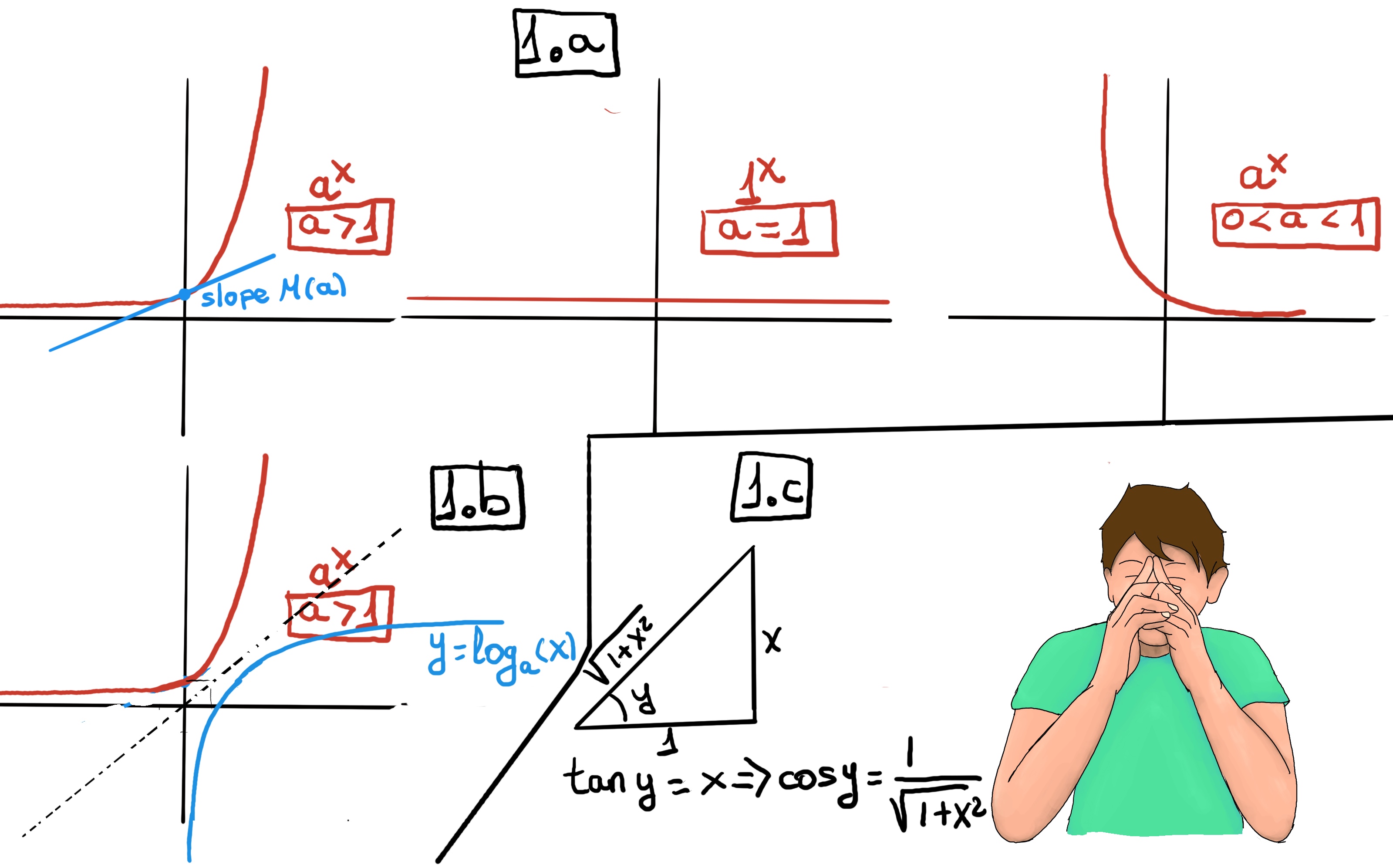
End Behaviour of exponential functions

An exponential function is a mathematical function of the form f(x) = b·a^x, where the independent variable appears in the exponent, and a and b are constants. The base a must be a positive real number (a > 0), and typically b > 0 as well..

Base Greater Than One (a > 1). When a > 1, the exponential function exhibits exponential growth (it can be observed that as the exponent increases, the curve get steeper). As x increases, f(x) heads to infinity (the function grows without bound), $\lim_{x \to ∞} a^x = ∞$. As x decreases, the function f(x) heads to or approaches zero, $\lim_{x \to -∞} a^x = 0$. Monotonicity: the exponential function is strictly increasing since (e^x)’ = e^x > 0, (a^x)’ = a^x·ln(a) > 0 for all x. The x-axis (y = 0) serves as a horizontal asymptote.
It is important to realize that as x approaches negative infinity, values become arbitrarily small but never actually reach zero, e.g., 2^-5 ≈ 0.03125, 2^-15 ≈ 0.00003052. Besides, the base of an exponential function determines the rate of growth or decay. For a > 1, the larger the base, the faster the function grows (Figure iii).
Base Between Zero and One (0 < a < 1). When 0 < a < 1, the exponential function exhibits exponential decay: As x increases, the function f(x) approaches zero, $\lim_{x \to ∞} a^x = 0$. As x decreases, the function grows without bond, $\lim_{x \to -∞} a^x = ∞$. Monotonicity: the function is strictly decreasing since $(a^x)' = a^x \ln(a) < 0$ for all x (note: ln(a) < 0 when 0 < a < 1) and has a horizontal asymptote along the x-axis (y = 0).
When a = 1, the function becomes constant: f(x) = 1^x = 1 for all x. The graph is a horizontal line at y = 1.

End Behaviour of logarithmic functions

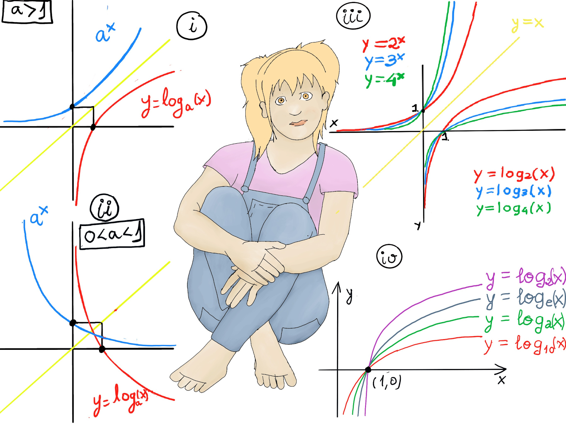
In mathematics, the logarithm is the inverse function to exponentiation. We call the inverse of a^x the logarithmic function with base a, that is, log_ax=y ↔ a^y=x. This means that the logarithm of a number x to the base a is the exponent to which a must be raised to produce x, e.g., log₄(64) = 3 ↭ 4³ = 64, log₂(16) = 4 ↭ 2⁴ = 16, log₈(512) = 3 ↭ 8³ = 512, but log₂(-3) is undefined (logarithms of negative numbers don’t exist in the real number system).

General Properties

As the inverse of exponential functions, logarithmic functions have the following characteristics:

The logarithm’s domain consists of real positive numbers.
Its range is ℝ (figure i and ii).
x-intercept: (1, 0), since log_a(1) = 0 for any base a; y-intercept: none (the function is undefined at x = 0).
Injectivity: It is one-to-one.
It has a vertical asymptote along the y-axis (x = 0).

Base Greater Than One (a > 1). It can be observed that as the value of the argument increases (x → ∞), the logarithm’s value grows without bound. As x increases, f(x) heads to infinity, $\lim_{x \to ∞} log_a(x) = \infin$. As x → 0⁺, the function approaches negative infinity, $\lim_{x \to 0+} log_a(x) = -\infin$. It is strictly increasing since $(\log_a(x))' = \frac{1}{x \ln(a)} > 0$ for all x > 0 and has a vertical asymptote along the y-axis (x = 0). The function passes through the point (1, 0) and increases slowly as x grows large.
The larger the base, the more slowly the logarithm grows. Equivalently, larger bases cause the graph to approach the vertical asymptote x = 0 more quickly. (Figure iii and iv).
Base Between Zero and One (0 < a < 1). As x → ∞, the function decreases without bound, $\lim_{x \to ∞} log_a(x) = -∞$. As x → 0⁺, the function approaches positive infinity, $\lim_{x \to 0+} log_a(x) = ∞$. Monotonicity. Strictly decreasing since $(\log_a(x))' = \frac{1}{x \ln(a)} < 0$ for all x > 0 (note: ln(a) < 0 when 0 < a < 1) and has a vertical asymptote along the y-axis (x = 0). The function still passes through (1, 0) but decreases as x increases.

Analysis and Plot of some functions

$\frac{1}{x}$ (Figure i).

Domain: $x \in \mathbb{R}, x \neq 0$
Range: $y \in \mathbb{R}, y \neq 0$
Symmetry: Odd function ($f(-x) = -f(x)$), symmetric about the origin.
Vertical asymptote: $\lim_{x \to 0⁺} \frac{1}{x} = +∞, \lim_{x \to 0⁻} \frac{1}{x} = -∞$ ⇒ x = 0 (y-axis) is a vertical asymptote.
Horizontal asymptote: $\lim_{x \to +∞} \frac{1}{x} = \lim_{x \to -∞} \frac{1}{x}= 0$ ⇒ y = 0 (x-axis) is a horizontal asymptote.
Some points to plot: $f(1) = 1, f(2) = 0.5, f(3) \approx 0.333, f(-1) = -1, f(-2) = -0.5, f(-3) \approx -0.333$.

We don’t have an expression for (ii). There is a horizontal asymptote, y = 1. As x approaches positive and negative infinity, there is a horizontal asymptote, y = 1, even though the function clearly passes through this line an infinite number of times.

A line y = L is a horizontal asymptote of f(x) if $\lim_{x \to +∞} f(x) = L$ and/or $\lim_{x \to -∞} f(x) = L$. In our particular case, L = 1, $\lim_{x \to +∞} f(x) = 1$ and $\lim_{x \to -∞} f(x) = 1$. Even though the function oscillates around y = 1 infinitely often for finite x, it eventually settles toward y = 1 as |x| becomes very large, e.g., $f(x) = 1 + \frac{sin(x)}{x}, g(x) = 1 + \frac{sin(x)}{x^2}$. The amplitude of oscillations decreases as |x| increases. For very large |x|, the function stays arbitrarily close to y = 1. Yet at many finite x-values, it crosses above and below y = 1.

$\frac{x+1}{x+3}$ (Figure iii).

Domain: $\mathbb{R} \setminus \{ -3 \}$ (denominator zero).
Range: $\mathbb{R} \setminus \{1 \}$ (y = 1, horizontal asymptote).
x-intercept: $x + 1 =0 \leadsto x=-1 \leadsto (-1, 0)$ y-intercept: $f(0) = \frac{0+1}{0+3} = \frac{1}{3}\leadsto (0, \frac{1}{3})$
Symmetry: None (not even or odd).
Asymptotes. $\lim_{x \to -3⁺} \frac{x+1}{x+3} = \frac{-2}{0⁻} = ∞, \lim_{x \to -3⁻} \frac{x+1}{x+3} = \frac{-2}{0⁺} = -∞$ ⇒ x = 3 is a vertical asymptote. $\lim_{x \to +∞} \frac{x+1}{x+3} = \lim_{x \to -∞} \frac{x+1}{x+3}= 1$ ⇒ y = 1 is a horizontal asymptote.
Direction of approach: As $x \to +\infty$: $f(x) = \frac{x+1}{x+3} = \frac{(x+3)-2}{x+3} = 1 - \frac{2}{x+3} < 1$ → approaches from below. As $x \to -\infty$: $\frac{2}{x+3} < 0$ for large negative x → $f(x) > 1$ → approaches from above.
Function Behavior Analysis. $f'(x) = \frac{2}{(x+3)^2} > 0$ for all $x \neq -3$. Therefore, function is increasing on both intervals $(-\infty, -3)$ and $(-3, \infty)$. Second Derivative: $f''(x) = -\frac{4}{(x+3)^3}$, $x < -3: (x+3)^3 < 0 \leadsto f''(x) > 0$ → concave up. $x > -3: (x+3)^3 > 0 \leadsto f''(x) < 0$ → concave down.
Two distinct branches: left branch (x < -3). Starts near y = 1 from above as $x \to -\infty$. Increases continuously while staying positive, concave up, approaches $+\infty$ as $x \to -3^-$, and lies entirely in quadrant II; right branch (x > -3). Approaches $-\infty$ as $x \to -3^+$. Increases continuously. Crosses x-axis at $(-1, 0)$ and y-axis at $(0, \frac{1}{3})$, concave down, approaches y = 1 from below as $x \to +\infty$.

Bibliography

This content is licensed under a Creative Commons Attribution-NonCommercial-ShareAlike 4.0 International License.

NPTEL-NOC IITM, Introduction to Galois Theory.
Algebra, Second Edition, by Michael Artin.
LibreTexts, Calculus. Abstract and Geometric Algebra, Abstract Algebra: Theory and Applications (Judson).
Field and Galois Theory, by Patrick Morandi. Springer.
Michael Penn, and MathMajor.
Contemporary Abstract Algebra, Joseph, A. Gallian.
YouTube’s Andrew Misseldine: Calculus. College Algebra and Abstract Algebra.
MIT OpenCourseWare 18.01 Single Variable Calculus, Fall 2007 and 18.02 Multivariable Calculus, Fall 2007.
Calculus Early Transcendentals: Differential & Multi-Variable Calculus for Social Sciences.